Sang-Heon Lee
This article explains how to estimate parameters of the linear regression model using the Bayesian inference. Our focus centers on user-friendly intuitive understanding of Bayesian estimation. From some radical point of view, we regard the Bayesian model as the average of multiple models generated with slightly different parameter set. We derive posterior distributions of parameters and perform estimation and simulation via Gibbs sampling using R code.
1. Introduction
Bayesian inference has been widely used to lots of research area such as VAR, DSGE, term structure model, state space model, and variable selection. There is also a tendency for incorporating Bayesian approach into machine/deep learnig techniques because Bayesian method also have characteristics of shrinkage and selection operation.
The purpose of this post is to present intuitive understanding of Bayesian modeling. This work will be a groundwork for advanced modeling like Bayesian estimation of VAR model or state-space model, and the dynamic Nelson-Siegel model.
The most important thing in Bayesian estimation is to take parameter uncertainty into account via prior distribution. It is quite useful to use Bayesian prior information when observation of data is small or structure of model is so complicated. Bayesian estimation tends to work well even when MLE is not working. It is also well known from a large number of existing studies that Bayesian foreasting is superior to traditional frequentist approach.
At first, let us know how to perform a estimation, forecast, simulation of a linear regression model using Bayesian approach.
For more detailed information, please refer to the following references. This aRticle is also written with the help of these references.
Blake, Andrew and Haroon Mumtaz, 2017. “Applied Bayesian Econometrics for Central Bankers”, Center for Central Banking Studies Technical Book.
Kang, Kyu Ho, 2016, Bayesian Econometrics, Pakyoungsa Publishing.
2. Bayesian Estimation
Bayesian estimation derives posterior distribution of parameters (\(\theta=parameters\)) based on the following Bayes theorem.
\[\begin{align} P(\theta|Y) = \frac{P(Y|\theta)P(\theta)}{P(Y)} \end{align}\]
At first, we need to calculate the likelihood function. The MLE estimation of linear regression is to maximize this likelihood function with respect to \(\beta\), \(\sigma^2\).
\[ F(Y_t | B,\sigma^2) = (2 \pi \sigma^2 )^{-\frac{T}{2}} e^{-\frac{(Y_t - X_t B)^{'}(Y_t - X_t B)}{2 \sigma^2}} \]
The distribution of parameter means that the number of parameter estimate is not one but many with probability density. As with the existing method, fixing a specific parameter to one estimate is very restrictive, so it is necessary to consider the uncertainty of the parameter. To account for parameter uncertainty, we assume some probabilty distribution for each parameters. After that, we use Bayes theorem to derive posterior distribution (\(H(B,\sigma^2 |Y_t )\)) from prior distribution or belief (\(P(B,\sigma^2 )\)) after observing data (\(F(Y_t |B,\sigma^2 )\)).
\[ H(B,\sigma^2 |Y_t )=\frac{F(Y_t |B,\sigma^2 )×P(B,\sigma^2 )}{F(Y_t )} \]
Here \(F(Y_t )\) is the density of data, marginal likelihood, marginal data density. \(F(Y_t )\) does not have parameters because they are integrated out. We can delete \(F(Y_t )\) since it is a constant scalar which only scales the sum of probability to one.
\[ H(B,\sigma^2 |Y_t ) ∝ F(Y_t |B,\sigma^2 )×P(B,\sigma^2 ) \]
3. Gibbs Sampling
Now let us estimate the linear regression model using Gibbs sampling which is one of the Bayesian MCMC approach.
Gibbs sampling is the method for drawing samples from posterior distribution when joint distribution \((\beta,\sigma^2|Y\)) is hard to calculate but each full conditional distributions are (\(\beta|Y,\sigma^2\)), (\(\sigma^2 |Y,\beta\)) which are easy to calculate. Continuing to sample from each full conditional distributions alternatively many times is the same to draw parameter samples from the joint distribution.
For example, given \(Y\),\(\sigma_0^2\), we draw \(\beta_1\). Using this sample (\(\beta_1\)) as input for \((\sigma^2 |Y,\beta)\), we draw \(\sigma_1^2\). This process results in first pair of parameters, \(( \beta_1,\sigma_1^2 )\). At second round, using \(\sigma_1^2\) as inptu for \((\beta|Y,\sigma^2)\), we draw \(\beta_2\). Using \(\beta_2\) as input for \((\sigma^2 |Y,\beta)\), we draw \(\sigma_2^2\). This process results in second pair of parameters, \((\beta_2,\sigma_2^2)\). Repeating this process n times, we can get \((\beta_1,\sigma_1^2 )\), \((\beta_2,\sigma_2^2 )\), … , \((\beta_n,\sigma_n^2)\).
Intuitively, sampling from each full conditional distribution will tend to draw samples from the support near to the average with some scarse draw of extreme values. Because it is of large errors in earlier sampling, we need to use samples after burn-in period.
4. Gibbs Sampling for Linear Regression
The following equation is a AR(2) model for Gibbs sampling.
\[\begin{align} Y_t&=\beta_0+\beta_1 Y_{t-1}+ \beta_2 Y_{t-2}+ \epsilon_t = X_t B + \epsilon_t \\ \epsilon_t &\sim N(0,\sigma^2 ) \end{align}\]
The procedure of Gibbs sampling is as follows.
Step 1) Assume prior distributions and set initial values
\[\begin{align} P(B)&\sim N(B_0,\Sigma_0 ) \\ &\sim N\left(\begin{bmatrix} \beta_0^0 \\ \beta_1^0 \\ \beta_2^0 \end{bmatrix} ,\begin{bmatrix} \Sigma_{\beta_0}&0&0 \\ 0&\Sigma_{\beta_1}&0 \\ 0&0&\Sigma_{\beta_2} \end{bmatrix} \right) \\ P(\sigma^2 )&\sim IG\left(\frac{T_0}{2},\frac{\theta_0}{2}\right) \end{align}\]
It is typical to use normal distributoin as a prior distribution for regression coefficients, which have real numbers. But for variance parameters which are always positive, inverse-gamma distribution is usually used. Two arguments of inverse-gamma distribution, \(T_0\) and \(\theta_0\), are shape and scale parameter respectively. The former is the degree of freedom which determines the height of distribution and the latter fixes the spread of it.
Step 2) Given initial value or previous draw of \(\sigma^2\), draw samples of \(B\) from the following conditional posterior distribution of \(B\).
\[\begin{align} &H(B| \sigma^2,Y_t ) \sim N(M^*,V^* ) \\ &\underbrace{M^* }_{3×1} = \left(\Sigma_0^{-1}+\frac{1}{\sigma^2} X_t^{'} X_t \right)^{-1} \left(\Sigma_0^{-1} B_0+\frac{1}{\sigma^2} X_t^{'} Y_t \right) \\ &\underbrace{V^* }_{3×3} = \left(\Sigma_0^{-1}+\frac{1}{\sigma^2} X_t^{'} X_t \right)^{-1} \end{align}\]
Step 3) Given value of \(B\), draw samples of \(\sigma^2\) from the following conditional posterior distribution of \(\sigma^2\).
\[\begin{align} &H(\sigma^2 |B,Y_t ) \sim IG \left(\frac{T_1}{2},\frac{\theta_1}{2}\right) \\ &T_1=T_0+T \\ &\theta_1=\theta_0+(Y_t - X_t B^1 )^{'} (Y_t - X_t B^1 ) \end{align}\]
Step 4) Repeating the above Step 2) and Step 3), we can get \((B^1,(\sigma^2 )^1 )\), \((B^2, (\sigma^2 )^2)\), …, \((B^M, (\sigma^2 )^M)\).
When M=5000 and burn-in=4000, we discard the first 4000 samples and take \((B^{4001},(\sigma^2 )^{4001})\), \((B^{4002},(\sigma^2 )^{4002})\), … , \((B^{5000},(\sigma^2 )^{5000})\). These are regarded as the final samples from the posteior distribution of \(B\) and \(\sigma^2\).
Means of \(B\) and \(\sigma^2\) are posterior mean respectively. The range between 5% and 95% of posterior samples is the 10% highest posterior density interval (HPDI) or credible set. If these HPDI does not contain 0, null hypothesis (\(B = 0\)) is rejected.
5. Derivation of Conditional Posterior Distributions
The following results are the derivation of conditional posteior distribution of parameters. Before delving into the derivation, we need to specifiy the likelihood function.
Likelihood function
\[\begin{align} F(Y_t |B,\sigma^2 ) &= (2\pi \sigma^2)^{\frac{T}{2}} e^{ -\frac{(Y_t-X_t B)^{'} (Y_t-X_t B)}{2\sigma^2}} \\ &∝ \exp \left( -\frac{(Y_t-X_t B)^{'} (Y_t-X_t B)}{2\sigma^2} \right) \end{align}\]
For sampling, we can delete \((2\pi \sigma^2)^{\frac{T}{2}}\) term in likelihood function because it does not affect relative density or sampling frequency.
Conditional posterior distribution of \(B\)
Prior distribution of \(B\) is assumed to follow the multivariate normal distribution.
\[\begin{align} P(B) &\sim N(B_0,\Sigma_0 ) \\ &\sim (2\pi)^{-\frac{K}{2}} |\Sigma_0 |^{-\frac{1}{2}} e^{-\frac{1}{2} (B-B_0 )^{'} \Sigma_0^{-1} (B-B_0 )} \\ P(B) &∝ \exp\left(-\frac{1}{2} (B-B_0 )^{'} \Sigma_0^{-1} (B-B_0 )\right) \end{align}\]
When \(\sigma^2\), \(Y_t\) are given, the conditional posterior distribution for \(B\) is propotional to the product of likelihood×prior.
\[\begin{align} & H(B|\sigma^2,Y_t ) \\ & ∝ \exp \left( -\frac{(Y_t-X_t B)^{'} (Y_t-X_t B)}{2\sigma^2} \right)\\ & \quad × \exp\left(-\frac{1}{2} (B-B_0 )^{'} \Sigma_0^{-1} (B-B_0 )\right) \\ & ∝ e ^{ -\frac{1}{2} \left( \frac{(Y_t-X_t B)^{'} (Y_t-X_t B)}{2\sigma^2} + (B-B_0 )^{'} \Sigma_0^{-1} (B-B_0 ) \right) } \end{align}\]
We can reduce the first term in RHS (\(\exp()\)) as follows.
\[\begin{align} & (Y_t-X_t B)^{'} (Y_t-X_t B) \\ & = Y_t^{'} Y_t - B^{'} X_t^{'} Y_t - Y_t^{'} X_t B + B^{'} X_t^{'} X_t B \\ & ∝ - 2 B^{'} X_t^{'} Y_t + B^{'} X_t^{'} X_t B \end{align}\]
Here \(- B^{'} X_t^{'} Y_t - Y_t^{'} X_t B =-2 B^{'} X_t^{'} Y_t\) because two scalar values are same. \(Y_t^{'} Y_t\) can be deleted since it is constant. These approach is also applied to the second term in RHS (\(\exp()\)).
\[\begin{align} & (B-B_0 )^{'} \Sigma_0^{-1} (B-B_0 ) \\ & = B^{'} \Sigma_0^{-1} B-B_0^{'} \Sigma_0^{-1} B-B^{'} \Sigma_0^{-1} B_0+B_0^{'} \Sigma_0^{-1} B_0 \\ & ∝ B^{'} \Sigma_0^{-1} B - 2 B_0^{'} \Sigma_0^{-1} B \end{align}\] Here \(B_0^{'} \Sigma_0^{-1} B-B^{'} \Sigma_0^{-1} B_0= -2 B_0^{'} \Sigma_0^{-1} B\) because two scalar values are same. \(B_0^{'} \Sigma_0^{-1} B_0\) can be deleted since it is constant. The final result is as follows.
\[\begin{align} & H(B|\sigma^2,Y_t ) \\ & ∝ e^ { -\frac{1}{2} (\frac{1}{\sigma^2} B^{'} X_t^{'} X_t B-2 \frac{1}{\sigma^2} B^{'} X_t^{'} Y_t+B^{'} \Sigma_0^{-1} B-2B^{'} \Sigma_0^{-1} B_0 )} \\ & ∝ e^ { -\frac{1}{2} (B^{'} (\Sigma_0^{-1}+\frac{1}{\sigma^2} X_t^{'} X_t )B-2B^{'} (\frac{1}{\sigma^2} X_t^{'} Y_t+\Sigma_0^{-1} B_0 ))} \\ & ∝ e^ { -\frac{1}{2} (B^{'} {V^*}^{-1} B-2B^{'} {V^*}^{-1} V^* (\frac{1}{\sigma^2} X_t^{'} Y_t+\Sigma_0^{-1} B_0 ))} \\ & ∝ e^ { -\frac{1}{2} (B^{'} {V^*}^{-1} B - 2B^{'} {V^*}^{-1} M^*) } \\ & ∝ N(M^*,V^* ) \\ \\ &M^* = \left(\Sigma_0^{-1}+\frac{1}{\sigma^2} X_t^{'} X_t \right)^{-1} \left(\Sigma_0^{-1} B_0+\frac{1}{\sigma^2} X_t^{'} Y_t \right) \\ &V^* = \left(\Sigma_0^{-1}+\frac{1}{\sigma^2} X_t^{'} X_t \right)^{-1} \end{align}\]
Conditional posterior distribution of \(\sigma^2\)
It is typical use normal distributoin as a prior distribution for regression coefficients, which have real number. But for variance parameter which is always positive, inverse-gamma distribution is usually used. Two arguments of inverse-gamma distribution, \(T_0\) and \(\theta_0\), are shape parameter and scale parameter. The former is the degree of freedom which determines the height of distribution. The latter fix the spread of distribution. We assume prior for variance parameter as the inverse-gamma (IG) distribution.
\[\begin{align} P(\sigma^2 ) \sim IG \left(\frac{T_0}{2},\frac{\theta_0}{2} \right) = (\sigma^2)^{-\frac{T_0}{2}-1} e^{-\frac{\theta_0/2}{\sigma^2}} \end{align}\]
When \(B\),\(Y_t\) are given, the conditional posterior distribution for \(\sigma^2\) is propotional to the product of likelihood and prior.
\[\begin{align} & H(\sigma^2 |B,Y_t ) \\ & ∝(\sigma^2 )^{-\frac{T}{2}} e^{-\frac{(Y_t-X_t B)^{'} (Y_t-X_t B)}{2 \sigma^2}} × (\sigma^2)^{-\frac{T_0}{2}-1} e^{-\frac{\theta_0/2}{\sigma^2}} \\ & ∝ (\sigma^2 )^{-\frac{T_0+T}{2}-1} e^{-\frac{1}{\sigma^2} \left( \frac{(Y_t-X_t B)^{'} (Y_t-X_t B) + \theta_0}{2} \right)} \\ & ∝ IG \left(\frac{T_1}{2},\frac{\theta_1}{2} \right) \\ \\ &T_1=T_0+T \\ &\theta_1=\theta_0+(Y_t - X_t B^1 )^{'} (Y_t - X_t B^1 ) \end{align}\]
6. R code for Gibbs sampling
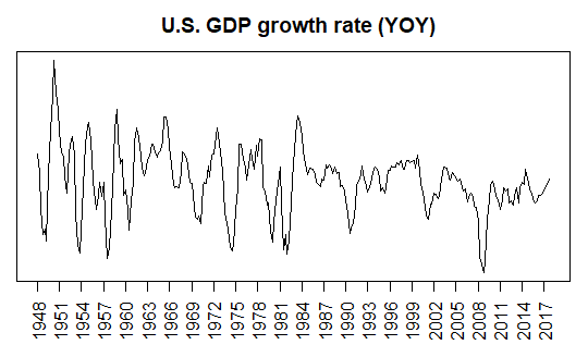
We can implement this Gibbs sampling algorithm for AR(2) model using the following R code. For data, we use U.S. quarterly GDP from the FRED database (https://fred.stlouisfed.org), which consists of two columns : date and GDP..
#=========================================================================# # Financial Econometrics & Derivatives, ML/DL using R, Python, Tensorflow # by Sang-Heon Lee # # https://shleeai.blogspot.com #-------------------------------------------------------------------------# # Bayesian linear regression using Gibbs sampling and Simulation # # Reference # # Blake, Andrew and Haroon Mumtaz, 2017. "Applied Bayesian econometrics # for central bankers," Center for Central Banking Studies Technical Book. # # Kang, Kyu Ho, 2016, "Bayesian Econometrics," Pakyoungsa Publishing. #=========================================================================# library(readxl) library(MASS) library(invgamma) graphics.off() # clear all graphs rm(list = ls()) # remove all files from your workspace setwd("D:/a_book_FIER_Ki_Lee/ch02_econ/bayesian") #----------------------------------------------------- # read data and transform yoy #----------------------------------------------------- # read data and extract dt df.data <- read_excel("US_GDP.xlsx","gdpc","A11:B305",col_names=TRUE) df.dt <- substr(df.data$observation_date,1,7) # yyyymm # YOY transform df.gdp.yoy <- log(df.data$GDPC1[5:nrow(df.data)] /df.data$GDPC1[1:(nrow(df.data)-4)]) df.dt.yoy <- df.dt[5:nrow(df.data)] nyoy <- length(df.gdp.yoy) # model scalar nlag <- 2 # lag nx <- 3 # number of X paramteres nhor <- 5*4 # h-ahead forecast niter <- 25000 # total numbers of Gibbs iterations nburn <- 15000 # percent of nburn-in iterations # Y, constant, Y(-1) Y(-2) df.yx.all <- data.frame(GDP = df.gdp.yoy[3:nyoy], const = 1, GDP_lag1 = df.gdp.yoy[2:(nyoy-1)], GDP_lag2 = df.gdp.yoy[1:(nyoy-2)]) df.dt.all <- df.dt.yoy[3:nyoy] # for x axis nall <- nrow(df.yx.all) # number of observations # spit sample is <- 1 # in-sample start ie <- nall - nhor # in-sample end os <- nall - nhor + 1 # out-of-sample start oe <- nall # out-of-sample end # in-sample for parameter estimation df.yx.is <- df.yx.all[is:ie,] df.dt.is <- df.dt.all[is:ie] # draw data x11(); plot(df.yx.is$GDP, xaxt='n', type="l", xlab="", ylab="GDP growth rate") axis(1, at=seq(1,ie-is-1,4), labels=substr(df.dt.is[seq(1,ie-is-1,4)],1,4), las=2) #----------------------------------------------------- # Gibbs sampling #----------------------------------------------------- Y <- as.matrix(df.yx.is[,1]) X <- as.matrix(df.yx.is[,-1]) T <- nrow(df.yx.is) x11(); plot(Y, type="l") #------------------------------------------ # step 1 : set priors and starting values #------------------------------------------ # initialization for priors B0 <- rep(0,nx) # priors for B Sigma0 <- diag(nx) # priors for sigma2 T0 <- 1; D0 <- 0.1 # priors for shape, scale of IG # starting values B <- B0; sigma2 <- 1 # output (parameters sampled) matrix m.out.param <- matrix(NA, niter - nburn,nx+1) colnames(m.out.param) <- c("beta1","beta2","beta3","sigma2") # to save forecast outputs m.out.forecast <- matrix(NA, nhor+nlag, niter - nburn) # Iterated sampling for (i in 1:niter) { print(paste(i,"-th iteration of total", niter, "........")) #--------------------------------------------- # step 2 : Draw B conditional on sigma2 #--------------------------------------------- V <- solve(solve(Sigma0) + (1/sigma2)*(t(X)%*%X)) M <- V%*%(solve(Sigma0)%*%B0 + (1/sigma2)*t(X)%*%Y) #check for stability chck=-1 while (chck<0) { # Draw B from N(M*,V*) B = t(t(mvrnorm(1,M,V))) # autoregressive matrix b=rbind(B[2:3,1],c(1, 0)) ee=max(abs(eigen(b)$values)) if (ee<=1 ) { chck=1 } } #--------------------------------------------- # step 3 : Sample sigma2 conditional on B #--------------------------------------------- resids=Y-X%*%B # residuals # posterior df and scale matrix T1=T0+T; D1=D0+t(resids)%*%resids # Draw sigma2 from IG(T1,D1) sigma2 = rinvgamma(1, T1, D1) # save a draw of (B, sigma2) pair for other purposes # after burn-in period if (i>nburn) { m.out.param[i-nburn,] <- c(as.numeric(B),sigma2) # 2-year forecast yhat <- matrix(0,nhor+nlag,1) yhat[1:2,1] <- Y[(nrow(Y)-1):nrow(Y),1] # starting values for (m in (nlag+1):(nhor+nlag)) { yhat[m,1] = cbind(1, yhat[m-1,1], yhat[m-2,1])%*%B + sqrt(sigma2)*rnorm(1) } m.out.forecast[,i-nburn] <- yhat } } #----------------------------------------------------- # Report output #----------------------------------------------------- # plot marginal posterior distributions x11(); par(mfrow=c(2,2)) for(i in 1:ncol(m.out.param)) { data <- m.out.param[,i] brks = seq(min(data),max(data),length.out=50) hist(data, main=colnames(m.out.param)[i], breaks = brks) } # the marginal posterior distribution of B m.out.beta <- m.out.param[,1:3] MB = apply(m.out.beta, 2, mean) # mean VB = apply(m.out.beta, 2, sd) # standard error EB = apply(m.out.beta, 2, # 95% error band function(x) { quantile(x,prob=c(0.05,0.95))}) m.results <- rbind(MB, VB, EB) print(m.results) # draw forecast FB = t(apply(m.out.forecast, 1, # percentiles function(x) { quantile(x,prob=c(9:1)*0.1)})) # concatenate historical data with forecast series m.out.Y.FB <- rbind(matrix(rep(Y,9),length(Y),9), FB[3:nrow(FB),]) # only foreast x11(); matplot(m.out.Y.FB, xaxt='n', yaxt='n',type="l", lty=1, ylim = c(min(df.yx.all$GDP), max(df.yx.all$GDP)), xlab="", ylab="", main="U.S. GDP growth rate (YOY)", ann = TRUE, lwd=1, col = 1:9) axis(1, at=seq(1,nall,12), labels=substr(df.dt.all[seq(1,nall,12)],1,4), las=2) # forecast with covid-19 growth rate x11(); matplot(m.out.Y.FB, xaxt='n', yaxt='n',type="l", lty=1, ylim = c(min(df.yx.all$GDP), max(df.yx.all$GDP)), xlab="", ylab="", main="U.S. GDP growth rate (YOY) with covid-19", ann = TRUE, lwd=1, col = 2:10) axis(1, at=seq(1,nall,12), labels=substr(df.dt.all[seq(1,nall,12)],1,4), las=2) lines(df.yx.all$GDP,type="l", lty=1, lwd=2) | cs |
7. Bayesian simulation and forecasting
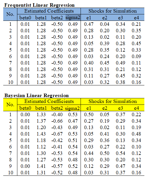
For simulation or forecasting, there is a striking difference between Frequentiest and Bayesian approach. As we know, typical simulation for linear regression use sequential random shocks. This random shock means the future uncertainty. But Bayesian simulation or forecasting consider not only future uncertainy but also parameter uncertainty. This lead to the different set of parameter estimates when simulation is repeated.
The following figure shows how different these two approach for simulation. For expositional purpose, number of simulation is set to 10. coefficient estimates (\(\beta_0\), \(\beta_1\), \(\beta_2\), \(\sigma^2\)) and 4-period random error (\(\epsilon_{t+h} \times 1000\), \(h=1,2,3,4\)) are reported.
In the above figure, the typical method at the top does not alter the estimated coefficient every when the number of simulations changes. This is something we are familiar with. However, if you look at the Bayesian method at the bottom of the figure above, it can be seen that the random error term changes as the number of simulations changes as in the typical method, but the estimated coefficients also change. That is, the set of estimated coefficients is sampled from the posterior distribution to take paramter uncertainty into account.
We give some radical interpretation : Frequentiest delivers one model but Bayesian so many models. For example, after Bayesian estimaiton, we can get 10000 set of parameters which form 10000 set of linear regression model. In this case, if 10000 paramter sets are determined randomly, it is useless. Therefore parameters follow certain joint distribution.
Probability distribution means that there are dense area (center of distribution) and coarse area (outside of distribution). Therefore, the characteristics of the parameter sets located at the center of the distribution will be somewhat similar, and the extreme cases which are located outside the distribution will be more different, but of course the number of extreme cases will be small.
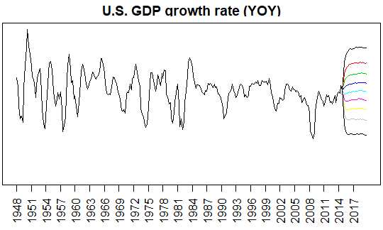
In the above R code, we reuse posterior sampling results for simulation. Simulaltion is performed for 20-quarter (5-year) horizon and 10000 iterations (=Total - burn-in = 25000 - 15000). From this simulaion result, we calculate the 9 percentiles (10%, 20%, ..., 80%, 90%) paths.
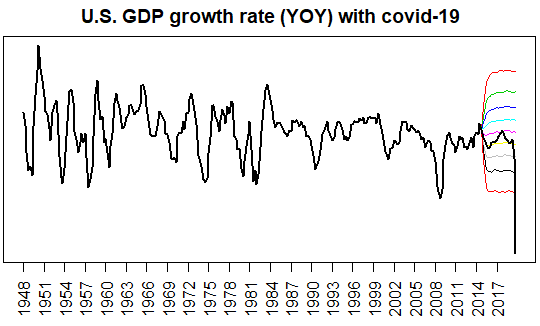
However, the recent impact of Covid-19 has caused a negative global growth shock, and the stress situation is still underway. In the following figure, out-of-sample GDP growth rate time series is plotted over the forecast period. It is not a dynamic forecast or a nowcast, but a five-year static forecast with a rather long forecast period, so there is a limitation in that the forecast error is large. Of course, very large stress shocks are unpredictable, so now is the time to predict whether they will get worse or back to the mean.
From this post we can understand Bayesian estimaiton, simulation, and forecasting. In particular we derive Gibbs sampling procedure and implement R code for this problem. Next post will cover some interesting but advanced topics such as Bayesian estimation of VAR, state-space model, and dynamic Nelson-Siegel model. \(\blacksquare\)


No comments:
Post a Comment