Understanding Hamilton Regime Switching Model using R package

This post explains how to implement a regime (Markov) switching model which is based on Hamilton (1989). The estimation is done by 1) predicting states by each regimes, 2) constructing a likelihood from data and state predictions, and 3) updating states. This is the Hamilton filter which is a kind of Bayesian updating procedure.

Hamilton Regime Switching Model

The recent rise in global inflation leads to the hit to living standards across the world. A recent article about this issue is as follows.

Prices paid by U.S. consumer jumped 7% in December from a year earlier, the highest inflation rate since 1982 and the latest evidence that rising costs for food, gas, rent and other necessities are heightening the financial pressures on America’s households. Inflation jumped at its fastest pace in nearly 40 years last month, a 7 percent spike from a year earlier that is pushing up household expenses, eating into wage gains and heaping pressure on President Joe Biden and the Federal Reserve to address a growing threat to the U.S. economy. Prices have risen sharply for cars, gas, food and furniture during a rapid recovery from the pandemic recession. Americans have ramped up spending amid shortages of workers and raw materials that have squeezed supply chains. .....

source : https://www.opb.org/article/2022/01/12/us-inflation-soared-7-in-past-year-the-most-since-1982/

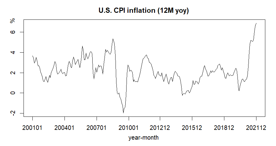
For this problem, we can think of regime switching behavior when we see the following U.S. CPI inflation (12M, yoy).

For this kind of asymmetric behavior of macro or financial variables, mostly used model is Hamilton (1989) regime switching model or its extension to state space model. In this post, let's understand the basic modeling approach using U.S. inflation data and a simple AR(1) model

Regime Switching model

Hamilton (1989) presents the regime switching model, which is so influential and is one of the main reference paper of so many academic papers. Let \(s_t = 0,1,2,...,k\) denotes the state variable with \(k\) regimes or states. In case of a two-state regime switching model, \(s_t = 0\) and \(s_t = 1\) can be interpreted as the expansion and recession states at time \(t\). A \(k\)-state linear regression model has the following form.

\[\begin{align} y_t &= c_{s_t} + \beta_{s_t}x_t + \epsilon_{s_t,t}, \quad \epsilon_{s_t,t} \sim N(0,\sigma_{s_t}) \\ &\quad \Downarrow \\ y_t &= c_1 + \beta_1 x_t + \epsilon_{1,t}, \quad \epsilon_{1,t} \sim N(0,\sigma_{1}) \\ y_t &= c_2 + \beta_2 x_t + \epsilon_{2,t}, \quad \epsilon_{2,t} \sim N(0,\sigma_{2}) \\ ... \\ y_t &= c_k + \beta_k x_t + \epsilon_{k,t}, \quad \epsilon_{k,t} \sim N(0,\sigma_{k}) \end{align}\]
Since \(s_t\) can take on 0, 1, ..., \(k\), a transition probability matrix is introduced to describe their transitions.

Markov Transition Probability Matrix

Each period, the regime or state follows Markov transition probability matrix. Markov means that transition probability depends on not long history of state transitions but only one lag. As examples, two- or three-state transition probability matrix are of the following forms.

two-state \[\begin{align} P(s_t=j|s_{t−1}=i) = P_{ij} = \begin{bmatrix} p_{00} & p_{01} \\ p_{10} & p_{11} \end{bmatrix} \end{align}\] three-state \[\begin{align} P(s_t=j|s_{t−1}=i) = P_{ij} = \begin{bmatrix} p_{00} & p_{01} & p_{02} \\ p_{10} & p_{11} & p_{12} \\ p_{20} & p_{21} & p_{22} \end{bmatrix} \end{align}\] where \(p_{ij}\) is the probability of transitioning from regime \(i\) at time \(t-1\) to regime \(j\) at time \(t\).

Inference about states with data

For simplicity, we take two-state regime (\(k=2\)). When \( \tilde{y}_t = \{y_1, y_2,..., y_{t-1}, y_t\}\) denotes an all available observations until time t and \(\mathbf{\theta} = \{c_1, c_2, \beta_1, \beta_2, \sigma_1, \sigma_2, p_{11}, p_{22}\}\) a vector of parameters an inference about the value of \(s_t\) based on the lastest observation \(y_t\).

\[\begin{align} \xi_{jt} &= P(s_t = j|\tilde{y}_t;\mathbf{\theta}) \\ &\quad \Downarrow \\ \xi_{0t} &= P(s_t = 0|\tilde{y}_t;\mathbf{\theta}) \\ \xi_{1t} &= P(s_t = 1|\tilde{y}_t;\mathbf{\theta}) \end{align}\]

This inference is our purpose. For this we use repeated predicting and updating procedures like the Kalman filter. When state transition is derived by state equation, we can use Kalman filter. But the state transition above is implemented as not state equation but state transition probability matrix. Under this transition environment, the Hamilton filter is for the inference about states with data and given parameters.

Hamilton Filtering

Hamilton filter is used to apply the state transition probabilities to construct the log-likelihood function. The Hamilton filter is similar to the Kalman filter with respect to the main Bayesian updating idea : repetitions of predicting and updating for state inference.

1) \(t-1\) state (previous state) \[\begin{align} \color{red}{\xi_{i,t-1}} &= P(s_{t-1} = i|\tilde{y}_{t-1};\mathbf{\theta}) \end{align}\] 2) state transition from \(i\) to \(j\) (state propagation) \[\begin{align} \color{blue}{p_{ij}} : \text{prob of i state at time t-1 to j state at time t} \end{align}\] 3) densities under the two regimes at \(t\) (data observations and state dependent errors) \[\begin{align} \color{green}{\eta_{jt}} &= f(y_t|s_t = j,\tilde{y}_{t-1};\mathbf{\theta}) \\ &= \frac{1}{\sqrt{2\pi}\sigma}\exp\left[-\frac{(y_t-c_j-\beta_j x_t)^2}{2\sigma_j^2}\right] \end{align}\] 4) conditional density of the time \(t\) observation (combined likelihood with state being collapsed): \(\quad\) a mix of 1) \(\rightarrow\) 2) \(\rightarrow\) 3) \[\begin{align} &f(y_t|\tilde{y}_{t-1};\mathbf{\theta}) \\ &= \sum_{i=1}^{2}{\sum_{j=1}^{2}{ \underbrace{ \overbrace{ \color{red}{\underbrace{\xi_{i,t-1}}_{\substack{\text{from i state} \\ \text{at time t-1}}}} \color{blue}{\underbrace{p_{ij}}_{\substack{\text{transition} \\ \text{from i to j}}}} }^{\text{forecast = prior}} \overbrace{ \color{green}{\underbrace{\eta_{jt}}_{\substack{\text{to j state} \\ \text{at time t}}}} }^{\text{data}} }_{\text{likelihood = prior ✕ data}} }} \\ &= \xi_{0,t-1}p_{00}\eta_{0t} + \xi_{0,t-1}p_{01}\eta_{1t} \\ &+ \xi_{1,t-1}p_{10}\eta_{0t} + \xi_{1,t-1}p_{11}\eta_{1t} \end{align}\] 5) \(t\) posterior state (corrected from previous state) \[\begin{align} \color{brown}{\xi_{jt}} &= P(s_t = j|\tilde{y}_t;\mathbf{\theta}) \\ &= \frac{\sum_{i=0}^{1} \xi_{i,t-1}p_{ij}\eta_{jt}} {f(y_t|\tilde{y}_{t-1};\mathbf{\theta})} \end{align}\] 6) use posterior state at time \(t\) as previous state a time \(t+1\) (substitution) \[\begin{align} \color{brown}{\xi_{jt}} \rightarrow \color{red}{\xi_{i,t-1}} \end{align}\] 7) iterate 1) ~ 6) from t = 1 to T

As a result of executing this iteration, the sample conditional log likelihood of the observed data can be calculated in the following way. \[\begin{align} \log f(\tilde{y}_{t}|y_0;\mathbf{\theta}) = \sum_{t=1}^{T}{ f(y_t|\tilde{y}_{t-1};\mathbf{\theta}) } \end{align}\] With this log-likelihood function, we use a numerical optimization to find the best fitting parameter set(\(\tilde{\mathbf{\theta}}\)).

R code

We implement R code for estimating two-state regime switching linear regression model and using R package. With U.S. CPI inflation (12M yoy) data ranging from 2001m01 to 20121m12, the following simple AR(1) model is estimated.

\[\begin{align} y_t = c_{s_t} + \beta_{s_t} y_{t-1} + \epsilon_{s_t,t}, \quad \epsilon_{s_t,t} \sim N(0,\sigma_{s_t}) \\ \end{align}\]
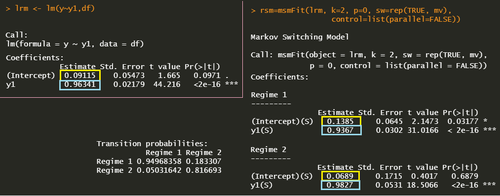
Since two-state model is used, parameters of interest are \(\mathbf{\theta} = c_1, c_2, \beta_1, \beta_2, \sigma_1, \sigma_2, p_{11}, p_{22} \). we use the msmFit() function of MSwM R package for the estimation of regime switching linear regression model. The msmFit() function takes linear regression results from lm() function as one of arguments.

#========================================================# # Quantitative ALM, Financial Econometrics & Derivatives  # ML/DL using R, Python, Tensorflow by Sang-Heon Lee  # # https://shleeai.blogspot.com #--------------------------------------------------------# # Hamilton Regime Switching Model - AR(1) inflation model #========================================================#   graphics.off()  # clear all graphs rm(list = ls()) # remove all files from your workspace   library(MSwM)   #------------------------------------------ # Data : U.S. CPI inflation 12M, yoy #------------------------------------------   inf <- c( 3.6536,3.4686,2.9388,3.1676,3.5011,3.144,2.6851,2.6851,2.5591, 2.1053,1.8767,1.5909,1.1888,1.13,1.3537,1.6306,1.2332,1.0635, 1.455,1.7324,1.5046,2.0068,2.2285,2.45,2.7201,3.0976,2.9804, 2.1518,1.8764,1.93,2.0347,2.1919,2.3505,2.0214,1.91,2.0148, 2.006,1.6744,1.7251,2.2667,2.8566,3.1185,2.8972,2.5155,2.5075, 3.1411,3.5576,3.2877,2.8052,3.0073,3.1565,3.3065,2.8289,2.5093, 3.0211,3.582,4.6328,4.2581,3.284,3.284,3.9401,3.5736,3.3608, 3.5501,3.9002,4.0967,4.0227,3.8514,1.9921,1.3965,1.9496,2.4927, 2.0545,2.3914,2.7598,2.5599,2.6738,2.6571,2.2914,1.8797,2.7944, 3.547,4.2803,4.0266,4.205,4.0594,3.8979,3.8295,4.007,4.818, 5.3517,5.1719,4.8345,3.6631,1.0939,-0.0222,-0.1137,0.0085,-0.4475, -0.578,-1.021,-1.2368,-1.9782,-1.495,-1.3875,-0.2242,1.8965,2.7753, 2.5873,2.1285,2.2604,2.1828,1.9837,1.1153,1.3319,1.1436,1.1121, 1.1599,1.0787,1.4276,1.6865,2.1026,2.5855,3.0308,3.4005,3.4424, 3.5173,3.6862,3.7417,3.4617,3.3932,3.0161,2.9644,2.857,2.5501, 2.2477,1.723,1.6403,1.4076,1.6719,1.931,2.1328,1.7801,1.7442, 1.67,1.998,1.5073,1.1324,1.3808,1.7012,1.8679,1.5271,1.0888, 0.873,1.2253,1.5015,1.5458,1.1142,1.5998,1.9951,2.1438,2.0381, 1.955,1.7006,1.67,1.5967,1.224,0.651,-0.2302,-0.0871,-0.022, -0.1041,0.035,0.1794,0.2254,0.241,0.0088,0.1275,0.4354,0.6367, 1.2299,0.8437,0.8877,1.1658,1.0727,1.0735,0.8646,1.0498,1.5368, 1.6719,1.6703,2.0301,2.4802,2.7167,2.3602,2.186,1.866,1.6498, 1.7255,1.9187,2.2042,2.0132,2.1872,2.0797,2.0722,2.2013,2.3318, 2.427,2.7149,2.7997,2.8511,2.6282,2.2586,2.4991,2.1768,1.902, 1.4846,1.461,1.8386,1.9981,1.8117,1.6863,1.8058,1.7261,1.7098, 1.7591,2.0231,2.2363,2.4441,2.2881,1.5004,0.3386,0.2233,0.7252, 1.0414,1.3161,1.4001,1.1876,1.1324,1.2918,1.3607,1.6618,2.6031, 4.0692,4.809,5.1876,5.1478,5.0717,5.2377,6.0564,6.6541,6.8811)     ninf <- length(inf)   # y and its first lag y0 <- inf[2:ninf]; y1 <- inf[1:(ninf-1)]  df <- data.frame(y = y0, y1 = y1)   #------------------------------------------ # Single State : OLS #------------------------------------------ lrm <- lm(y~y1,df) summary(lrm)   #------------------------------------------ # Two State : Markov Switching (MSwM) #------------------------------------------   k  <- 2 # two-regime mv <- 3 # means of 2 variables + 1 for volatility rsm=msmFit(lrm, k=2, p=0, sw=rep(TRUE, mv),                 control=list(parallel=FALSE)) summary(rsm)   # graphs with regime probabilities: x11(); plotProb(rsm,which=1) # filtered/smoothed prob x11(); plotProb(rsm,which=2) # regime 1 prob & shaded area x11(); plotProb(rsm,which=3) # regime 2 prob & shaded area   Colored by Color Scripter

cs

The estimation results below show that parameters of the single regime or standard AR(1) model are located between parameters of the two-regime switching model. Although the underlying model is a simple AR(1) model, it can capture some regime dependent bahavior of inflation.

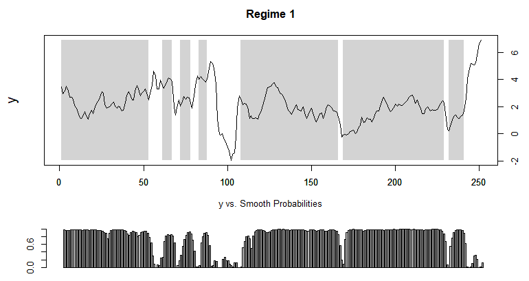
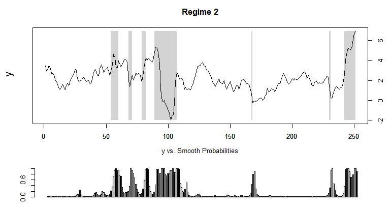
Now we can investigate two-regime probabilities by using plotProb() function in MSwM R package. As we expected we can identify two-regime : low or high volatility, in other words, slow or abrupt change. Of course, our simple regime switching AR(1) model does not capture directions and levels of inflation.

In particular, we can think that recent regime change from low to high inflation volatility (change) happens from 2021m03.

Concluding Remarks

In this post, we explains Hamilton regime switching model by taking AR(1) model as an example and implement R code with the help of MSwM R package. Hamilton filter is a kind of Bayesian updating procedure. Next time we will implement the same model by MLE for a deeper understanding of Hamilton regime switching model.

Reference

Hamilton, J. D. (1989) A New Approach to the Economic Analysis of Nonstationary Time Series and the Business Cycle. Econometrica 57, pp. 357–384. \(\blacksquare\)