This post shows how to use rjags R package to perform Bayesian MCMC estimation. As an example, we just select a multiple linear regression but rjags can handle lots of highly non-linear models so that it can be extended to various modelings including hierarchical models.

Bayesian Estimation by using rjags Package

JAGS is the abbreviation for Just Another Gibbs Sampler which is used for easy Bayesian modeling. rjags is a kind of wrapper of jags. This post will use rjags R package to estimate a multiple linear regression model by Bayesian MCMC. Prior to installing rjags, jags should be installed at first.

https://sourceforge.net/projects/mcmc-jags/

Likelihood

The likelihood of a multiple linear regression model (k=2) is constructed from the following model specification. \((t=1,2,…,n)\)

\[\begin{align} Y_t &\sim \text{Normal}(\mu, \tau) \\ \mu &= \beta_0+\beta_1 X_{1t}+\beta_2 X_{2t} \\ \sigma &= 1/\sqrt{\tau} \end{align}\]
Here, \(\tau\) in \(\text{Normal}(\mu, \tau)\) is not a variance but a precision which is the reciprocal of a variance (\(\tau = \frac{1}{\sigma^2}\)).

Prior

Priors for regression coefficients and the reciprocal of an error variance should be given. Although there is no 'true' prior distribution, there is a 'satisficing' prior distribution. It can be done by a lot of experience or from the previous studies.

In our case, \(\beta\) are assumed to have normal priors but \(\tau\) is non-negative and is assumed to have a gamma prior. We use \(\hat{\beta_0}, \hat{\beta_1}, \hat{\beta_2}\) which are OLS estimates as each mean of priors for regression coefficients. Precision is set to 0.01 to represent our confidence is moderate and is not strong.

\[\begin{align} \beta_0 &\sim \text{Normal}(\hat{\beta_0}, 0.01) \\ \beta_1 &\sim \text{Normal}(\hat{\beta_1}, 0.01) \\ \beta_2 &\sim \text{Normal}(\hat{\beta_2}, 0.01) \\ \tau &\sim \text{Gamma}(0.01, 0.01) \end{align}\]
To use rjags, we have only to define model and each prior for coefficients without any lengthy derivations.

Model String in rjags

In rjags, a main part is a model string which consists of a likelihood and priors (with or without transformations). It is the same as the above equations essentially. When our model (likelihood) or priors are changed, we need to modify this model string properly.

"
model{
    # likelihood
    for( i in 1:n) {
        y[i] ~ dnorm(mu[i], tau)
        mu[i] <- beta0 +beta1*x[i,1] + beta2*x[i,2]
    }
    
    # priors
    beta0 ~ dnorm(b_guess[1], 0.1)
    beta1 ~ dnorm(b_guess[2], 0.1)
    beta2 ~ dnorm(b_guess[3], 0.1)  
    tau   ~ dgamma(.01,.01)
    
    # transform
    sigma <- 1 / sqrt(tau)
}
" 
 

R code

As an example, we take an AR(2) model as a test model. Data is the U.S. quarterly GDP growth rate (yoy) ranging from 1947Q1 to 2019Q1. In the next R code, jags.script is the model string.

1
2
3
4
5
6
7
8
9
10
11
12
13
14
15
16
17
18
19
20
21
22
23
24
25
26
27
28
29
30
31
32
33
34
35
36
37
38
39
40
41
42
43
44
45
46
47
48
49
50
51
52
53
54
55
56
57
58
59
60
61
62
63
64
65
66
67
68
69
70
71
72
73
74
75
76
77
78
79
80
81
82
83
84
85
86
87
88
89
90
91
92
93
94
95
96
97
98
99
100
101
102
103
104
105
106
107
108
109
110
111
112
113
114
115
116
117
118
119
120
121
122
123
124
125
126
127
128
129
130
131
132
133
134
135
136
137
138
139
140
141
142
143
144
145
146
147
148
149
150
151
152
153
154
155
156
157
158
159
160
161
162
163
164
165
166
167
168
169
170
#========================================================#
# Quantitative ALM, Financial Econometrics & Derivatives 
# ML/DL using R, Python, Tensorflow by Sang-Heon Lee 
#
# https://shleeai.blogyield.com
#--------------------------------------------------------#
# rjags example for Bayesian multiple regression
#========================================================#
graphics.off(); rm(list = ls())
 
library(rjags)
library(coda)
 
#-----------------------------------------------------
# read data (U.S. quarterly GDP growth rate year-on-year)
#-----------------------------------------------------
 
# quarterly data for U.S. GDP growth rate (yoy)
gdp_yoy <-c(
  0.0257139670,  0.0447562683,  0.0525359910,  0.0381317790,  0.0093259088,
 -0.0104627119, -0.0059041116, -0.0154490719,  0.0369748307,  0.0704341513,
  0.0980788417,  0.1254736302,  0.1004152961,  0.0875517208,  0.0700361239,
  0.0532694875,  0.0504080513,  0.0353806505,  0.0221731143,  0.0522873341,
  0.0600764198,  0.0656249942,  0.0527893859,  0.0052196433, -0.0179898299,
 -0.0246006338, -0.0077274628,  0.0269059373,  0.0598597082,  0.0749112146,
  0.0770952717,  0.0637027107,  0.0316489075,  0.0237374609,  0.0094243285,
  0.0197643323,  0.0300394541,  0.0196166557,  0.0302665177,  0.0035414395,
 -0.0291434042, -0.0203977878, -0.0072740159,  0.0262493878,  0.0715814738,
  0.0873426752,  0.0651795264,  0.0449022299,  0.0480956652,  0.0203738001,
  0.0245428618,  0.0087791174, -0.0067174527,  0.0155233387,  0.0296569900,
  0.0619956746,  0.0729468622,  0.0651106689,  0.0583064298,  0.0421683677,
  0.0353464754,  0.0375090926,  0.0470449534,  0.0502963040,  0.0603030182,
  0.0599724792,  0.0537286165,  0.0502782228,  0.0533241329,  0.0550495076,
  0.0615364189,  0.0812312602,  0.0813724980,  0.0722292596,  0.0586735114,
  0.0440647570,  0.0288308733,  0.0260330499,  0.0270165087,  0.0263581712,
  0.0377310270,  0.0536885532,  0.0519915518,  0.0484049473,  0.0437450686,
  0.0302104821,  0.0290740384,  0.0202599426,  0.0032441293,  0.0016268587,
  0.0042170031, -0.0016684843,  0.0266150980,  0.0305934387,  0.0296160568,
  0.0427453445,  0.0341702075,  0.0512175143,  0.0524209432,  0.0666718926,
  0.0728962552,  0.0612801001,  0.0466076021,  0.0394491207,  0.0063674420,
 -0.0020862905, -0.0063096723, -0.0196461231, -0.0232590023, -0.0185129237,
  0.0079550988,  0.0252192903,  0.0597054841,  0.0598956257,  0.0483960934,
  0.0422431855,  0.0317503644,  0.0436947211,  0.0561051726,  0.0489047254,
  0.0403457494,  0.0590058015,  0.0511281571,  0.0644582144,  0.0630677430,
  0.0262218823,  0.0236181481,  0.0127638331,  0.0141078278, -0.0077808984,
 -0.0163713694, -0.0003914969,  0.0158731684,  0.0292547991,  0.0423481003,
  0.0129153625, -0.0221468644, -0.0101568967, -0.0258912833, -0.0145366869,
  0.0142131192,  0.0321625248,  0.0557863013,  0.0760345142,  0.0823011467,
  0.0769304925,  0.0667314613,  0.0542590241,  0.0445441428,  0.0361798193,
  0.0417411642,  0.0409714759,  0.0406189998,  0.0363467080,  0.0307157148,
  0.0286666689,  0.0267990197,  0.0330364855,  0.0321503663,  0.0438187584,
  0.0415476345,  0.0438695504,  0.0410730401,  0.0372852235,  0.0422469583,
  0.0367975587,  0.0383368666,  0.0270684337,  0.0278223606,  0.0238411639,
  0.0171246753,  0.0060106594, -0.0095473822, -0.0054029478, -0.0010277132,
  0.0115967019,  0.0281855548,  0.0312037714,  0.0359977334,  0.0428964179,
  0.0326695847,  0.0276917220,  0.0226193094,  0.0257511647,  0.0337339603,
  0.0413861313,  0.0424524751,  0.0403331370,  0.0342190216,  0.0237385166,
  0.0263811775,  0.0217583082,  0.0256785859,  0.0392405346,  0.0396996610,
  0.0432626787,  0.0422360126,  0.0421785102,  0.0456794827,  0.0439007010,
  0.0474109873,  0.0401430518,  0.0401600330,  0.0476381748,  0.0471132023,
  0.0455598811,  0.0461236331,  0.0469470314,  0.0411378962,  0.0516217468,
  0.0399447798,  0.0293013196,  0.0228343952,  0.0105169266,  0.0050232471,
  0.0015336818,  0.0130966573,  0.0133071719,  0.0219020499,  0.0207290678,
  0.0175542787,  0.0200810319,  0.0324846821,  0.0423539093,  0.0421448528,
  0.0411709185,  0.0337402858,  0.0322909355,  0.0379764716,  0.0349895931,
  0.0344545645,  0.0307824359,  0.0329887855,  0.0307180626,  0.0233893470,
  0.0255771428,  0.0147141403,  0.0180922467,  0.0219651225,  0.0195425692,
  0.0114268306,  0.0108650373,  0.0000187657, -0.0279169036, -0.0334437760,
 -0.0400352950, -0.0309725345,  0.0018270714,  0.0169579334,  0.0275769043,
  0.0312874776,  0.0253699929,  0.0191222715,  0.0170685309,  0.0094456342,
  0.0159653298,  0.0261720704,  0.0233405632,  0.0249669608,  0.0145788777,
  0.0155972048,  0.0125376209,  0.0189926726,  0.0258053859,  0.0141565704,
  0.0263693756,  0.0307011415,  0.0283625033,  0.0406403469,  0.0339376821,
  0.0254217778,  0.0214119574,  0.0176133228,  0.0139843073,  0.0157940174,
  0.0204649433,  0.0204575407,  0.0216035638,  0.0234362726,  0.0266744034,
  0.0303073105,  0.0327109848,  0.0306872928,  0.0244537329,  0.0224051369)
 
ndata <- length(gdp_yoy)
 
# Y, Y(-1) Y(-2)
df.yx <- data.frame(GDP = gdp_yoy[3:ndata], 
                    GDP_lag1 = gdp_yoy[2:(ndata-1)], 
                    GDP_lag2 = gdp_yoy[1:(ndata-2)])
 
#-----------------------------------------------------
# regression by using lm
#-----------------------------------------------------
lm_est <- lm(GDP ~ ., data = df.yx)
 
 
#-----------------------------------------------------
# Bayesian regression by using rjags
#-----------------------------------------------------
 
# Prepare data and additional information(n)
lt.Data <- list(x = df.yx[,-1], y = df.yx[,1],
                n = nrow(df.yx))
 
# for use additional information(b_guess) inside model
lt.Data$b_guess <- lm_est$coefficients
 
# Model string
jags.script <- 
"#--------------------------------------------------
model{
    # likelihood
    for( i in 1:n) {
        y[i] ~ dnorm(mu[i], tau)
        mu[i] <- beta0 +beta1*x[i,1] + beta2*x[i,2]
    }
    # priors
    beta0 ~ dnorm(b_guess[1], 0.1)
    beta1 ~ dnorm(b_guess[2], 0.1)
    beta2 ~ dnorm(b_guess[3], 0.1)  
    tau   ~ dgamma(.01,.01)
    
    # transform
    sigma <- 1 / sqrt(tau)
}#--------------------------------------------------
" 
 
# compile
mod1 <- jags.model(textConnection(jags.script), 
                   data = lt.Data, 
                   n.chains = 4, n.adapt = 1000)
# run
update(mod1, 4000)
 
# posterior sampling
mod1.samples <- coda.samples(
    model = mod1, 
    variable.names = c("beta0", "beta1", "beta2", "sigma"), 
    n.iter = 2000)
 
# plot trace and posterior density for each parameter
x11(); plot(mod1.samples)  
# descriptive statistics of posterior densities
sm <- summary(mod1.samples); sm
# correlation
cor(mod1.samples[[1]])
 
 
#-----------------------------------------------------
# mean parameters
#-----------------------------------------------------
# means of posteriors of parameters
beta0.post.mean <- sm$statistics["beta0", "Mean"]
beta1.post.mean <- sm$statistics["beta1", "Mean"]
beta2.post.mean <- sm$statistics["beta2", "Mean"]
sigma.post.mean <- sm$statistics["sigma", "Mean"]
 
beta_post <- rbind(beta0.post.mean,
                   beta1.post.mean,
                   beta2.post.mean,
                   sigma.post.mean)
 
# real data and fitted values
ypred <- as.matrix(cbind(1,df.yx[,-1]))%*%beta_post[-4]
 
x11(width = 16/2, height = 9/2)
matplot(cbind(ypred,df.yx[,1]), type=c("l","p"), pch = 16,
        lty=c(1,1), lwd=3, col=c("blue", "green"))
 
# Frequentist and Bayesian coefficients
coefs <- rbind(c(lm_est$coefficients, sigma(lm_est)), 
               t(beta_post))
colnames(coefs) <- c("const", "beta1", "beta2", "sigma")
rownames(coefs) <- c("Frequentist", "Bayesian")
coefs
 
Colored by Color Scripter
cs

Except for jags.script, the remaining part is not changed. In particular, it is worth noting that variables in jags.script should be in lt.Data like

lt.Data$b_guess <- lm_est$coefficients
cs

.
Therefore when additional variables should be used in model string (jags.script), we should add that variables into that data list (lt.Data).

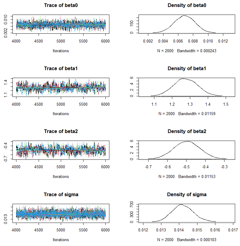
Estimation results contain of the following posterior distributions for each parameters.

Bayesian Estimation by using rjags Package R code

A summary statistics and average of posteriors can be obtained in the following way.

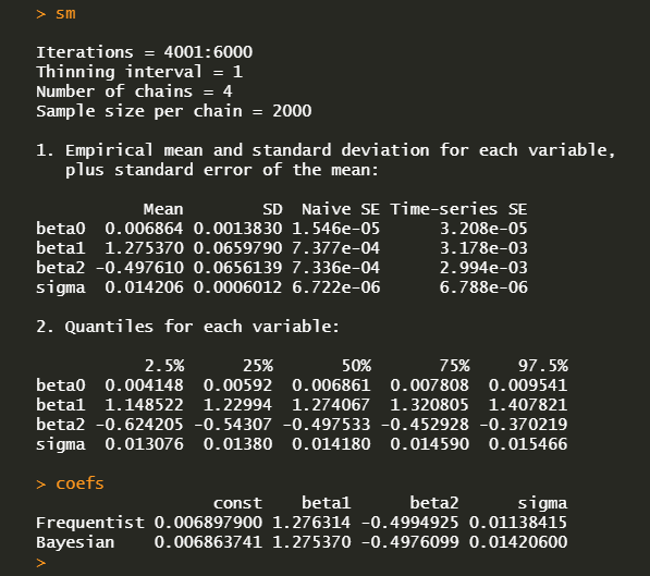
We can generate a time series of fitted response variable with average coefficients.

Concluding Remarks

This post shows how to use rjags R package to perform Bayesian MCMC estimation with multiple linear regression example. This is an easy tool for Bayesian analysis for us only if we understand the meaning of hyper-parameters of various prior distributions and use them without hesitation. \(\blacksquare\)

SHLee AI Financial Model

Pages

Bayesian Estimation by using rjags R Package