Paste R plot image into MS Word with additional information
The officer R package makes an access to and manipulates 'Microsoft Word' and 'Microsoft PowerPoint' documents from R. Specifically, R objects such as a plot image, string and so on can are pasted into MS Word or PowerPoint.
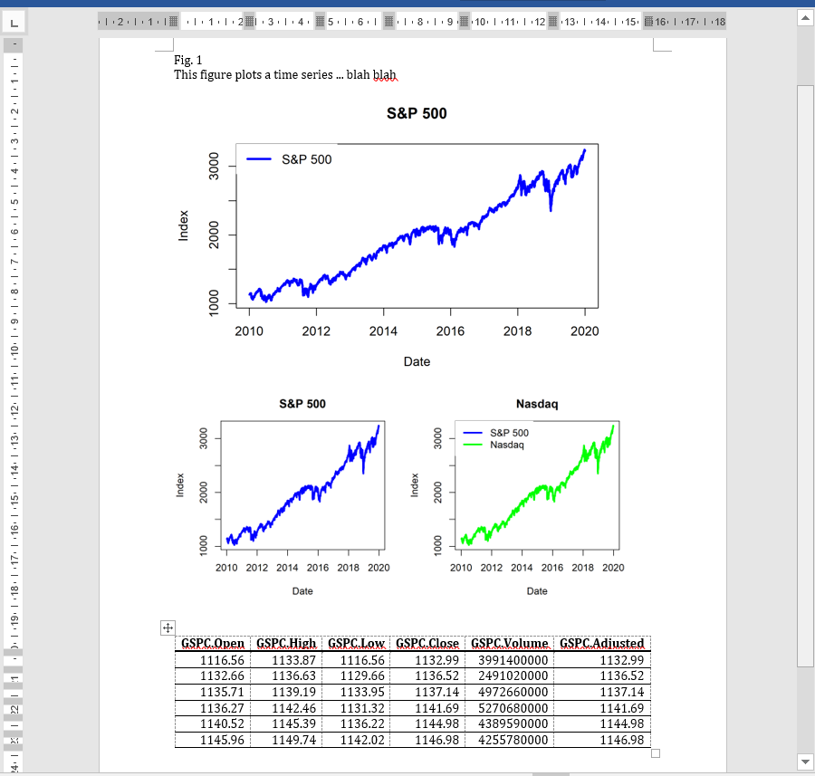
The focus of this post centers on pasting R plot images into Word as follows.
Useful functions of officer R package
How to use the officer R package consists of the following structure.
1 2 3 4 5 | doc <- read_docx() doc <- body_add(doc, ....) print(doc, target = filename) | cs |
First, read_docx() function create an internal Word object and return it.
Second, by calling body_add() function with different arguments (...) several times as needed, a variety of contents are pasted into Word. The arguments (...) is dependent on which type of R components are considered. For example, the argument for a plot and that of a table (data.frame) are as follows respectively.
1 2 3 4 5 | doc <- body_add(doc, dataframe, style = "table_template") doc <- body_add(doc, plot_instr( code = barplot(1:5, col = 2:6))) | cs |
For a plot image, body_add() function takes graph-generating codes with plot_instr() sub component.
Finally print() function save the internal Word object as a file with a user-defined filename. For more detailed information, please see the manual of the officer R package. It provides many useful examples.
R code
The following R code pastes plot images into MS Word with a title, description, and data table. I show two cases by using direct commands or a function encapsulating that commands.
1 2 3 4 5 6 7 8 9 10 11 12 13 14 15 16 17 18 19 20 21 22 23 24 25 26 27 28 29 30 31 32 33 34 35 36 37 38 39 40 41 42 43 44 45 46 47 48 49 50 51 52 53 54 55 56 57 58 59 60 61 62 63 64 65 66 67 68 69 70 71 72 73 74 75 76 77 78 79 80 81 82 83 84 85 86 87 88 89 90 91 92 93 94 95 96 97 98 99 100 101 102 103 104 105 106 107 108 109 110 111 112 113 114 115 116 117 118 119 120 | #========================================================# # Quantitative Financial Econometrics & Derivatives # ML/DL using R, Python, Tensorflow by Sang-Heon Lee # # https://shleeai.blogspot.com #--------------------------------------------------------# # Paste plot images to MS Word #========================================================# graphics.off(); rm(list = ls()) library(quantmod) # getSymbols library(officer) setwd("D:") #------------------------------------------------ # read S&P 500 and NASDAQ index #------------------------------------------------ sdate <- as.Date("2010-01-01") edate <- as.Date("2020-01-01") getSymbols("^GSPC", from=sdate, to=edate) getSymbols("^IXIC", from=sdate, to=edate) df <- data.frame( time(GSPC[,6]), GSPC[,6], IXIC[,6]) rownames(df) <- NULL colnames(df) <- c("date", "GSPC", "NDAQ") #----------------------------------------------------------- # draw graph by direct commands #----------------------------------------------------------- # figure 1 x11(width=16/2, height=5) matplot(df$date, df$GSPC, main = "S&P 500", type = "l", lwd = 3, col = "blue", xlab="Date", ylab="Index") legend('topleft',legend="S&P 500", col="blue", lty=1,lwd=3, box.lty=0) # figure 2 x11(width=16/2, height=5) par(mfrow=c(1,2), mar = c(6, 4, 3, 2)) # bltr matplot(df$date, df$GSPC, main = "S&P 500", type = "l", lwd = 3, col = "blue" , xlab="Date", ylab="Index") matplot(df$date, df$GSPC, main = "Nasdaq" , type = "l", lwd = 3, col = "green", xlab="Date", ylab="Index") legend('topleft',legend=c("S&P 500", "Nasdaq"), col=c("blue", "green"), lty=1,lwd=3, box.lty=0) #----------------------------------------------------------- # graph function #----------------------------------------------------------- f_draw_one <- function(x, y, title) { matplot(x, y, main = title, type = "l", lwd = 3, col = "blue", xlab="Date", ylab="Index") legend('topleft',legend=title, col="blue", lty=1,lwd=3, box.lty=0) } f_draw_two <- function(x1, y1, title1, x2, y2, title2) { par(mfrow=c(1,2), mar = c(6, 4, 3, 2)) # bltr matplot(x1, y1, main = title1, type = "l", lwd = 3, col = "blue" , xlab="Date", ylab="Index") matplot(x2, y2, main = title2 , type = "l", lwd = 3, col = "green", xlab="Date", ylab="Index") legend('topleft',legend=c(title1, title2), col=c("blue", "green"), lty=1,lwd=3, box.lty=0) } # draw figure 1 and 2 using functions x11(width=16/2, height=5) f_draw_one(df$date, df$GSPC, "S&P 500") x11(width=16/2, height=5) f_draw_two(df$date, df$GSPC, "S&P 500", df$date, df$GSPC, "Nasdaq") #----------------------------------------------------------- # paste images to a WORD file with additional information #----------------------------------------------------------- ### create a new document object doc <- read_docx() ### add title and description doc <- body_add(doc, "Fig. 1", style = "Normal") desc <- "This figure plots a time series ... blah blah" doc <- body_add(doc, desc, style = "Normal") ### various method to add figure into WORD # 1) by direct commands doc <- body_add(doc, plot_instr(code = { matplot(df$date, df$GSPC, main = "S&P 500", type = "l", lwd = 3, col = "blue", xlab="Date", ylab="Index") legend('topleft',legend="S&P 500", col="blue", lty=1,lwd=3, box.lty=0) }), height = 4) # 2) by encapsulated function doc <- body_add(doc, plot_instr(code = { f_draw_two(df$date, df$GSPC, "S&P 500", df$date, df$GSPC, "Nasdaq") }), width = 8, height = 4) ### add table if necessary doc <- body_add(doc, "", style = "Normal") doc <- body_add(doc, head(as.data.frame(GSPC)), style = "table_template") ### save word file print(doc, target="r_to_word_test.docx") | cs |
The output Word file (r_to_word_test.docx) is the first figure in this post, which is located at a working directory(in our case, D:/). With the help of the manual for the officer R package, you can use more useful functionalities than this post.
No comments:
Post a Comment