Tibshirani (1996) introduces the so called LASSO (Least Absolute Shrinkage and Selection Operator) model for the selection and shrinkage of parameters. This model is very useful when we analyze big data. In this post, we learn how to set up the Lasso model and estimate it using glmnet R package.
Tibshirani (1996) introduces the LASSO (Least Absolute Shrinkage and Selection Operator) model for the selection and shrinkage of parameters. The Ridge model is similar to it in terms of the shrinkage but does not have selection function because the ridge model make the coefficient of unimportant variable close to zero but not exactly to zero.
These regression models are called as the regularized or penalized regression model. In particular, Lasso is so powerful that it can work for big dataset in which the number of variables is more than 100 or 1000, 10000, .... and so on. The traditional linear regression model cannot deal with this sort of big data.
Although the linear regression estimator is the unbiased estimator in terms of bias-variance trade-off relationship, the regularized or penalized regression such as Lasso, Ridge admit some bias for reducing variance. This means the minimization problem for the latter has two components: mean squared error and penalty for parameters. \(l_1\)-penalty of Lasso make variable selection and shrinkage possible but \(l_2\)-penalty of Ridge make only shrinkage possible.
Model : Lasso
For observation index \(i=1,2,...,N\) and variable index \(j=1,2,...,p\), standardized predictors \(x_{ij}\) and demeaned or centered response variables) are given, Lasso model finds \(\beta_j\) which minimize the following objective function.
\[\begin{align} \text{Linear Regression} &: \sum_{i=1}^{N} { \left(y_i-\sum_{j=1}^{p}x_{ij}\beta_j \right)^2} \\ \text{Lasso Regression} &: \sum_{i=1}^{N} { \left(y_i-\sum_{j=1}^{p}x_{ij}\beta_j \right)^2} + \lambda \sum_{j=1}^{p} |\beta_j| \\ \text{Ridge Regression} &: \sum_{i=1}^{N} { \left(y_i-\sum_{j=1}^{p}x_{ij}\beta_j \right)^2} + \lambda \sum_{j=1}^{p} {\beta_j}^2 \end{align}\]
Here, \(Y\) is demeaned for the sake of exposition, but this is not a must. However, X variables should be standardized with mean zero and unit variance because the difference in scale of variables tends to distribute penalty to each variables unequally.
From the above equations, the first part of it is the RSS (Residual Sum of Squares) and the second is the penalty term. This penalty term is adjusted by the hyperparameter \(\lambda\). Hyperparameter is given exogenously by user through the process of mannual searching or cross-validation.
When certain variable is included in the Lasso but decreases RSS so small to be negligible (i.e. decreasing RSS by 0.000000001), the impact of the shrinkage penalty grows. This means the coefficient of this variable is to zero (Lasso) or close to zero (Ridge).
Unlike the Ridge (convex and differentiable), the Lasso (non-convex and non-differentiable) does not have the closed-form solution in most problems and we use the cyclic coordinate descent algorithm. The only exception is the case where all X variables are orthonormal but this cas is highly unlikely.
R code
Let's estimate parameters of Lasso and Ridge using glmnet R package which provides fast calculation and useful functions.
For example, we make some articial time series data. let\(X\) be 10 randomly drawn time series (variables) and \(Y\) variable with predetermined coefficients and randomly drawn error terms. Some coefficient are set to zero for the clear understanding of the differences between the standard linear, Lasso, and Ridge regression. The R code is as follows.
1 2 3 4 5 6 7 8 9 10 11 12 13 14 15 16 17 18 19 20 21 22 23 24 25 26 27 28 29 30 31 32 33 34 35 36 37 38 39 40 41 42 43 44 45 46 47 48 49 50 51 52 53 54 55 56 57 58 59 60 61 62 63 64 65 66 67 68 69 70 71 72 73 74 75 76 77 78 79 80 81 82 83 84 85 86 87 88 89 90 91 92 93 94 95 96 97 98 99 100 101 102 103 104 105 106 107 108 109 110 111 112 113 114 115 116 117 118 119 120 121 122 123 124 125 126 127 128 129 130 131 132 133 134 135 | #=========================================================================# # Financial Econometrics & Derivatives, ML/DL using R, Python, Tensorflow # by Sang-Heon Lee # # https://shleeai.blogspot.com #-------------------------------------------------------------------------# # Lasso, Ridge #=========================================================================# library(glmnet) graphics.off() # clear all graphs rm(list = ls()) # remove all files from your workspace N = 500 # number of observations p = 20 # number of variables #-------------------------------------------- # X variable #-------------------------------------------- X = matrix(rnorm(N*p), ncol=p) # before standardization colMeans(X) # mean apply(X,2,sd) # standard deviation # scale : mean = 0, std=1 X = scale(X) # after standardization colMeans(X) # mean apply(X,2,sd) # standard deviation #-------------------------------------------- # Y variable #-------------------------------------------- beta = c( 0.15, -0.33, 0.25, -0.25, 0.05,rep(0, p/2-5), -0.25, 0.12, -0.125, rep(0, p/2-3)) # Y variable, standardized Y y = X%*%beta + rnorm(N, sd=0.5) y = scale(y) #-------------------------------------------- # Model #-------------------------------------------- lambda <- 0.01 # standard linear regression without intercept(-1) li.eq <- lm(y ~ X-1) # lasso la.eq <- glmnet(X, y, lambda=lambda, family="gaussian", intercept = F, alpha=1) # Ridge ri.eq <- glmnet(X, y, lambda=lambda, family="gaussian", intercept = F, alpha=0) #-------------------------------------------- # Results (lambda=0.01) #-------------------------------------------- df.comp <- data.frame( beta = beta, Linear = li.eq$coefficients, Lasso = la.eq$beta[,1], Ridge = ri.eq$beta[,1] ) df.comp #-------------------------------------------- # Results (lambda=0.1) #-------------------------------------------- lambda <- 0.1 # lasso la.eq <- glmnet(X, y, lambda=lambda, family="gaussian", intercept = F, alpha=1) # Ridge ri.eq <- glmnet(X, y, lambda=lambda, family="gaussian", intercept = F, alpha=0) df.comp <- data.frame( beta = beta, Linear = li.eq$coefficients, Lasso = la.eq$beta[,1], Ridge = ri.eq$beta[,1] ) df.comp #------------------------------------------------ # Shrinkage of coefficients # (rangle lambda input or without lambda input) #------------------------------------------------ # lasso la.eq <- glmnet(X, y, family="gaussian", intercept = F, alpha=1) # Ridge ri.eq <- glmnet(X, y, family="gaussian", intercept = F, alpha=0) # plot x11(); par(mfrow=c(2,1)) x11(); matplot(log(la.eq$lambda), t(la.eq$beta), type="l", main="Lasso", lwd=2) x11(); matplot(log(ri.eq$lambda), t(ri.eq$beta), type="l", main="Ridge", lwd=2) #------------------------------------------------ # Run cross-validation & select lambda #------------------------------------------------ mod_cv <- cv.glmnet(x=X, y=y, family='gaussian', intercept = F, alpha=1) # plot(log(mod_cv$lambda), mod_cv$cvm) # cvm : The mean cross-validated error # - a vector of length length(lambda) # lambda.min : the λ at which # the minimal MSE is achieved. # lambda.1se : the largest λ at which # the MSE is within one standard error # of the minimal MSE. x11(); plot(mod_cv) coef(mod_cv, c(mod_cv$lambda.min, mod_cv$lambda.1se)) print(paste(mod_cv$lambda.min, log(mod_cv$lambda.min))) print(paste(mod_cv$lambda.1se, log(mod_cv$lambda.1se))) | cs |
Estimation Results
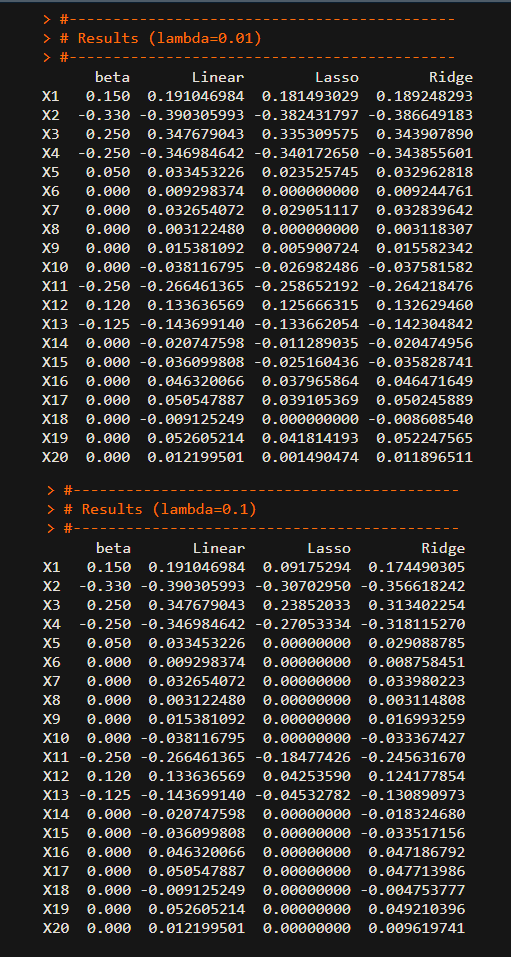
The following figure shows true coefficients (\(\beta\)) with which we generate data, the estimated coefficients of three regressoin models.
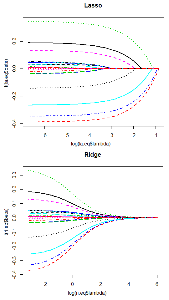
The estimation results provide similar results between models despite the uncertainty in data-generating process. In particular, Lasso is identifying the insignificant or unimportant variables as zero coefficients. The variable selection and shrinkage effect are strong with \(\lambda\). The following figures show the change of estimated coefficients with respect to the change of the penalty parameter (\(log(\lambda)\)) which is the shrinkage path.
Model Selection
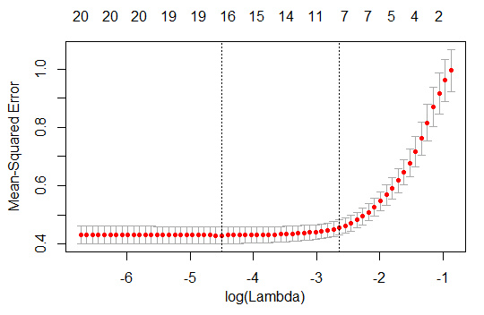
The most important thing in Lasso boils down to select the optimal \(\lambda\). This is determined in the process of the cross-validation. cv.glmnet() function in glmnet provides the cross-validation results with some proper range of \(\lambda\). Using this output, we can draw a graph of \(log(\lambda)\) and MSE(measn squared error).
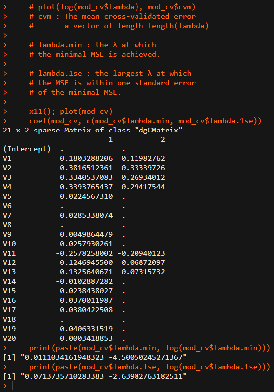
From the above figures, the first candiate is the \(\lambda\) at which the minimal MSE is achieved but it is likely that this model have many variables. The second is the largest \(\lambda\) at which the MSE is within one standard error of the minimal MSE. This is somewhat heuristic or empirical approach but have some merits for reducing the number of variables. It is typical to choose the second, MSE minimized 1se \(\lambda\). But visual inspection is very important tool to find the pattern of shrinkage process.
The following result reports the estimated coefficients under the MSE minimized \(\lambda\) and MSE minimized 1se \(\lambda\) respectively.
Forecast
After estimating the parameters of Lasso regression, it is necessary to use this model for prediction. The forecasting exercise use not the penalty term but the estimated coefficients. Looking at the forecasting method, the Lasso, Ridge, and linear regression models are the same because the penalty term is only used for the estimation.
Based on this post, sign restricted Lasso model will be discussed. It is important to set constraints on the sign of coefficient since the economic theory or empirical stylized fact advocate the specific sign.
Tibshirani, Robert (1996). "Regression Shrinkage and Selection via the lasso," Journal of the Royal Statistical Society 58-1, 267–88. \(\blacksquare\)


No comments:
Post a Comment