It is a stylized fact that the default risk decreases in GDP growth rate, but increase in GDP growth volatility. This relationship is empirical and theoretical guideline for the model selection. Therefore, all explanatory variables should be consistent to its own expected signs.
The lasso, ridge, and linear regression model is the unrestricted model as default setting. But The sign restrictions need to be included as additional constraints in optimization problem. Implementing this optimization problem is not easy but we can sidestep this difficulty by using glmnet R package.
Since the following R code have a self-contained structure, it is easy to understand. In this code, The expected signs of each coefficients are given by user as following rule.
- 1 : expected sign is plus(+)
- -1 : expected sign is mimus(-)
- 0 : expected sign is indeterminate
1 2 3 4 5 6 7 8 9 10 11 12 13 14 15 16 17 18 19 20 21 22 23 24 25 26 27 28 29 30 31 32 33 34 35 36 37 38 39 40 41 42 43 44 45 46 47 48 49 50 51 52 53 54 55 56 57 58 59 60 61 62 63 64 65 66 67 68 69 70 71 72 73 74 75 76 77 78 79 80 81 82 83 84 85 86 87 88 89 90 91 92 93 94 95 96 97 98 99 100 101 102 103 104 105 106 107 | #===================================================================# # Financial Econometrics & Derivatives, ML/DL, R,Python,Tensorflow # by Sang-Heon Lee # # https://shleeai.blogspot.com #-------------------------------------------------------------------# # Sign constrained Lasso, Ridge, Stnadard Linear Regression #===================================================================# library(glmnet) graphics.off() # clear all graphs rm(list = ls()) # remove all files N = 500 # number of observations p = 20 # number of variables #-------------------------------------------- # X variable #-------------------------------------------- X = matrix(rnorm(N*p), ncol=p) # before standardization colMeans(X) # mean apply(X,2,sd) # standard deviation # scale : mean = 0, std=1 X = scale(X) # after standardization colMeans(X) # mean apply(X,2,sd) # standard deviation #-------------------------------------------- # Y variable #-------------------------------------------- beta = c( 0.15, -0.33, 0.25, -0.25, 0.05, rep(0, p/2-5), -0.25, 0.12, -0.125, rep(0, p/2-3)) # Y variable, standardized Y y = X%*%beta + rnorm(N, sd=0.5) y = scale(y) #-------------------------------------------- # Model without Sign Restrictions #-------------------------------------------- # linear regression without intercept( using -1) li.eq <- lm(y ~ X-1) # linear regression using glmnet li.gn <- glmnet(X, y, lambda=0, family="gaussian", intercept = F, alpha=0) # lasso la.eq <- glmnet(X, y, lambda=0.05, family="gaussian", intercept = F, alpha=1) # Ridge ri.eq <- glmnet(X, y, lambda=0.05, family="gaussian", intercept = F, alpha=0) #-------------------------------------------- # Model with Sign Restrictions #-------------------------------------------- # Assign Expected sign as arguments of glmnet v.sign <- sample(c(1,0,-1),p,replace=TRUE) vl <- rep(-Inf,p); vu <- rep(Inf,p) for (i in 1:p) { if (v.sign[i] == 1) vl[i] <- 0 else if (v.sign[i] == -1) vu[i] <- 0 } # linear regression using glmnet with sign restrictions li.gn.sign <- glmnet(X, y, lambda=0, family="gaussian", intercept = F, alpha=1, lower.limits = vl, upper.limits = vu) # lasso with sign restrictions la.eq.sign <- glmnet(X, y, lambda=0.05, family="gaussian", intercept = F, alpha=1, lower.limits = vl, upper.limits = vu) # Ridge with sign restrictions ri.eq.sign <- glmnet(X, y, lambda=0.05, family="gaussian", intercept = F, alpha=0, lower.limits = vl, upper.limits = vu) #-------------------------------------------- # Results #-------------------------------------------- df.out <- as.data.frame(as.matrix(round( cbind(li.eq$coefficients, li.gn$beta, li.gn.sign$beta, la.eq$beta, la.eq.sign$beta, ri.eq$beta, ri.eq.sign$beta),4))) # for clarity df.out[df.out==0] <- "." df.out <- cbind( ifelse(v.sign==1,"+",ifelse(v.sign==-1,"-",".")), ifelse(v.sign==1,"plus",ifelse(v.sign==-1,"minus",".")), df.out) # always important to use appropriate column names colnames(df.out) <- c("Sign", "Desc", "Linear.lm", "Linear", "Linear.Sign","Lasso", "Lasso.Sign", "Ridge", "Ridge.Sign") print(df.out) | cs |
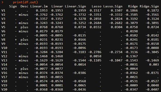
From the above estimation results, we can find that estimated coefficients are consistent with each expected sign. When estimated sing conflicts with the expected one, its coefficients is set to zero and is discarded. Therefore we can understand that the sign restrictions is another form of variable selection process which reduce more the range of selected variables.
Generally speaking, it is not easy to impose the expected sign restrictions but we can do it with powerful glmnet R package.\(\blacksquare\)

No comments:
Post a Comment