Markowitz v.s. Michaud Portfolio Optimization with R code

This post shows how to perform asset allocation based on the Markowitz's mean-variance (MV) portfolio model which is the benchmark framework. This model is based on the diversification effect. Another alternative Michaud's Resampled Efficiency (RE) portfolio model is also discussed. These two models are implemented using a quadratic optimization R library.

Introduction

It is, however, cautious to apply MV model to practical problems because MV have some limitations such as error maximization or corner solution. This is regarded as serious problems since the diversification effect, which is the purpose of the portfolio optimization, is not achieved.

There are lots of alternative approaches to circumbent these problems. Michaud, inter alia, suggests the Resampled Efficiency (RE) portfolio model. This model is similar to Random Forest model but is not difficult to implement.

Michaud, Richard and Robert Michaud, 2007. “Estimation Error and Portfolio Optimization:A Resampling Solution”, New Frontier Advisors

Mean-Variance Portfolio Optimization Problem

Markowitz formulates mean-variance portfolio optimization problem as follows.

\[\begin{align} & min_{w} ⁡\frac{1}{2} w^{'}\Sigma w \\ & s.t. \\ & w^{'} [1,1,…,1]^{'} = 1 \\ & w ≥ 0 \\ & E(r)= w^{'} \mu \end{align}\]

Here, \(w\), \(\mu\), \(\Sigma\) denote weights vector, expected return vector, covariance matrix respectively. \(E(r)\) is a given target return.

The solution of the above problem is the optimal weight vector which minimizes the portfolio variance \((w^{'}\Sigma w )\) while attaining a given target expected return. This type of model is called as the quadratic programming and is solved using QP solver.

Resampled Portfolio Optimization Problem

Resampled portfolio (RE portfolio) uses the simulation sheme for generating th samples of expected return vector and covariance matrix as follows.

1. Use the expected return and covariance matrix as input for multivariate normal distribution.
2. From 1)'s multivariate normal distribution, simulate asset returns.
3. From 2)'s simulated asset returns, calculate the mean and covariance matrix again.
4. Using 3)'s mean and covariance matrix, run MV optimization.
5. After iterating 1), 2), 3), 4) steps N times, calculate the average weight vector.

solveQPXT() function

Let's use R to perform MV and RE QP portfolio optimization. To solve a quadratic programming, we use the solveQPXT() function from the quadprogXT R package. The prototype of this function is as follows.
solveQPXT(Dmat,dvec,Amat,bvec,meq=0,factorized=FALSE)

Since the above specification of function is mapped to the following equations, we only need to know how to relate them.
\[\begin{align} & min_{w} \frac{1}{2} b^{'} D b - d^{'} b \\ & s.t. \\ & A^{'} b ≥ b_0 \end{align}\]

Data

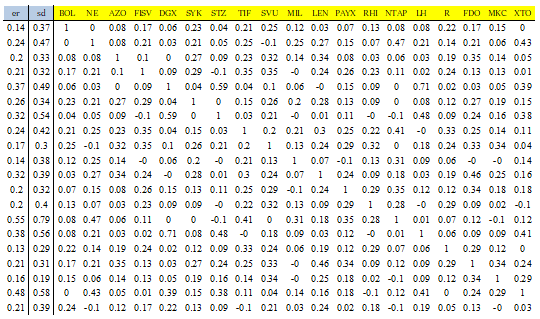
For empirical analysis, we use Michaud (2007) paper's data which consists of the average, standard deviation, correlation of 20 asset classes.

R code for Portfolio optimization

R code for portfolio optimization 1) reads data, 2) perform MV portfolio optimization, and 3) RE portfolio optimization sequentially. Data can be downloaded at : mu_sd_corr_michaud.csv

#=========================================================================#
# Financial Econometrics & Derivatives, ML/DL using R, Python, Tensorflow  
# by Sang-Heon Lee
#
# https://shleeai.blogspot.com
#-------------------------------------------------------------------------#
# Resampled Portfolio Optimization
#
# Reference
#
# Estimation Error and Portfolio Optimization:A Resampling Solution 
# - Richard Michaud and Robert Michaud
#
# https://www.newfrontieradvisors.com/media/1138/estimation-error
# -and-portfolio-optimization-12-05.pdf
#=========================================================================#

graphics.off()  # clear all graphs
rm(list = ls()) # remove all files from your workspace

library(quadprogXT) # solveQPXT
library(MASS)       # mvrnorm

#-----------------------------------------------------
# Michuad dataset
#-----------------------------------------------------

    setwd("D:/a_book_FIER_Ki_Lee/ch09_Portfolio/resampled")

    # This dataset exists in appendix of Michaud and Michaud (2007)
    df.data <- read.csv('mu_sd_corr_michaud.csv')
    head(df.data)
    
    # mean, std, correlation
    mu   <- as.vector(df.data[,1])
    sd   <- as.vector(df.data[,2])
    corr <- as.matrix(df.data[,-c(1,2)])
    
    # number of asset
    nvar <- length(mu)
    var.name <- colnames(df.data[,-c(1,2)])
    
    # convert correlation to covariance matrix
    cov <- diag(sd)%*%corr%*%diag(sd)

#-----------------------------------------------------
# Traditional portfolio optimization
#-----------------------------------------------------
    
    n.er <- 100  # number of EF points
    rset <- seq(min(mu),max(mu),length=n.er+2)
    rset <- rset[2:n.er+1]
    
    port1.ret <- rset
    port1.std <- rset*0
    port1.wgt <- matrix(0,n.er,nvar)
    
    # calculate efficient frontier
    for (i in 1:n.er) {
        Dmat <- 2*cov
        dvec <- rep(0,nvar) #c(0,0)
        Amat <- t(rbind(t(rep(1,nvar)),t(mu),diag(nvar)))
        bvec <- c(1,rset[i],rep(0,nvar))
        
        # mean-variance optimization
        m<-solveQPXT(Dmat,dvec,Amat,bvec,meq=2,factorized=FALSE)
        
        # output
        port1.std[i]  <- sqrt(m$value)
        port1.wgt[i,] <- t(m$solution)
    }
    
    # draw efficient fronter and allocation profile
    x11(width=6); par(mfrow = c(2,1), mar = c(3,2,2,3), xpd=TRUE)
    
        # individual asset
        plot(sqrt(diag(cov)), mu,
             xlim=c(0.8*min(port1.std),1.2*max(port1.std)), 
             ylim=c(0.8*min(mu),1.2*max(mu)),
             col = rainbow(nvar), lwd = 10)
        text(sqrt(diag(cov)), mu, 
             labels=var.name, cex= 1)
        
        # efficient frontier
        lines(port1.std,port1.ret,col = "green", lwd = 6)
        
        # weight
        barplot(t(port1.wgt),col=rainbow(nvar))
        legend("topright", legend = var.name,
               fill = rainbow(nvar), ncol = 1,
               inset=c(-0.07,0), cex = 0.6)
        
#-----------------------------------------------------
# Resampled portfolio optimization
#-----------------------------------------------------
        
    n.er <- 100  # number of EF points
    rset <- seq(min(mu),max(mu),length=(n.er+2))
    rset <- rset[2:(n.er+1)]
        
    port.re.ret <- rset
    port.re.std <- rset*0
    port.re.wgt <- matrix(0,n.er,nvar)
        
    n.rr = 1000  # number of resampling
        
    for (rr in 1:n.rr) {
        print(rr)
        
        # simulated time series of assets
        sim     <- mvrnorm(n = 120, mu, cov)
            
        # simulated mu & cov
        mu.sim  <- colMeans(sim)
        cov.sim <- cov(sim)
            
        rset.sim <- seq(min(mu.sim),max(mu.sim),length=(n.er+2))
        rset.sim <- rset.sim[2:(n.er+1)]
            
        port.sim.ret <- rset.sim
        port.sim.std <- rset.sim*0
        port.sim.wgt <- matrix(0,n.er,nvar)
        
        # calculate efficient frontier
        for (i in 1:n.er) {
            Dmat <- 2*cov.sim
            dvec <- rep(0,nvar) 
            Amat <- t(rbind(t(rep(1,nvar)),t(mu.sim),diag(nvar)))
            bvec <- c(1,rset.sim[i],rep(0,nvar))
                
            # mean-variance optimization
            m<-solveQPXT(Dmat,dvec,Amat,bvec,meq=2,factorized=FALSE)
                
            # output
            port.sim.std[i]  <- sqrt(m$value)
            port.sim.wgt[i,] <- t(m$solution)
        }  
            
        # sum of resampling portfolios before average
        port.re.ret <- port.re.ret + port.sim.ret
        port.re.wgt <- port.re.wgt + port.sim.wgt
    }
        
    # average of resampling portfolios
    port.re.wgt <- port.re.wgt/n.rr
    port.re.ret <- port.re.ret/n.rr
        
    # portfolio SD and Expexted Return 
    for (i in 1:n.er) {
        port.re.ret[i] <- port.re.wgt[i,]%*%mu
        port.re.std[i] <- sqrt(port.re.wgt[i,]%*%cov%*%port.re.wgt[i,])
    }
        
    # draw efficient fronter and allocation profile
    x11(width=6); par(mfrow = c(2,1), mar = c(3,2,2,3), xpd=TRUE)
    
        # individual asset
        plot(sqrt(diag(cov)), mu,
             xlim=c(0.8*min(port1.std),1.2*max(port1.std)),
             ylim=c(0.8*min(mu),1.2*max(mu)),
             col = rainbow(nvar), lwd = 10)
        text(sqrt(diag(cov)), mu,
             labels=colnames(df.data[,3:22]), cex= 1)
        
        # efficient frontier
        lines(port1.std,     port1.ret,col = "green" , lwd = 10)
        lines(port.re.std, port.re.ret,col = "blue", lwd = 4)
        
        
        # weight
        barplot(t(port.re.wgt),col=rainbow(nvar))
        legend("topright", legend = var.name,
               fill = rainbow(nvar), ncol = 1,
               inset=c(-0.07,0), cex = 0.6)
               

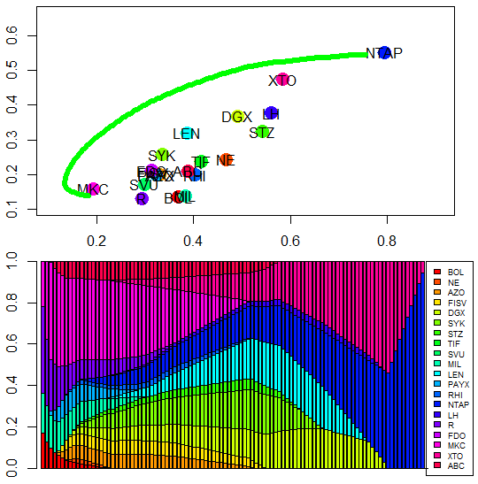
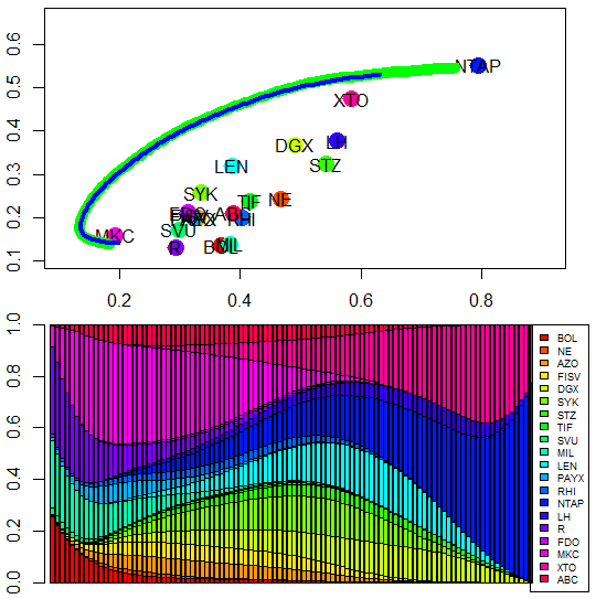
Running this R code draw the efficient frontier of MV portfolio and allocation weights profile as follows.

Efficient frontier is the standard deviation and expected return's locus of minimum variance portfolio with varying target expected returns. Rational investor selects the optimal portfolio on the efficient frontier according to his/her attitude of risk and return or risk appetite. As I mentioned earlier, we can find the abrupt changes of allocations which reduce the diversification effect.

However, we can find that allocation weights of RE portfolio generate the smoother changes than that of MV portoflio. This means weight chagnes of RE portoflio are not too sensitive unlike MV portfolio.

From these results, we learn MV and RE portoflio optimization model. Typcally, RE model is preferred to MV model because RE model delivers more diversified allocation and has the tendency to show the higher Sharpe ratio empirically or heuristically.

Next post will cover several important asset allocation models such as , Black-Litterman (BL) which incorporate market view into MV model, regime-switching portfolio optimization, dynamic portfolio optimization, and Machine / Deep Learning based portfolio optimization model, and so on. \(\blacksquare\)