Cross Validation in Lasso : Binomial Response
Cross validation for lasso is provided by glmnet R package and we can use it easily. Nevertheless, is there any reason why we implement cross validation procedure manually?. In a cross-sectional context, we just use cv.glmnet() function in glmnet R package without hesitation.
But when we deal with time-series data, it is often necessary to implement the process of cross validation (forward chaining) manually due to the lack of similar built-in functions. Therefore, if we replicate results of cv.glmnet(), we can modify this results for use in another purposes such as time series data analysis, especially variable selection using lasso.
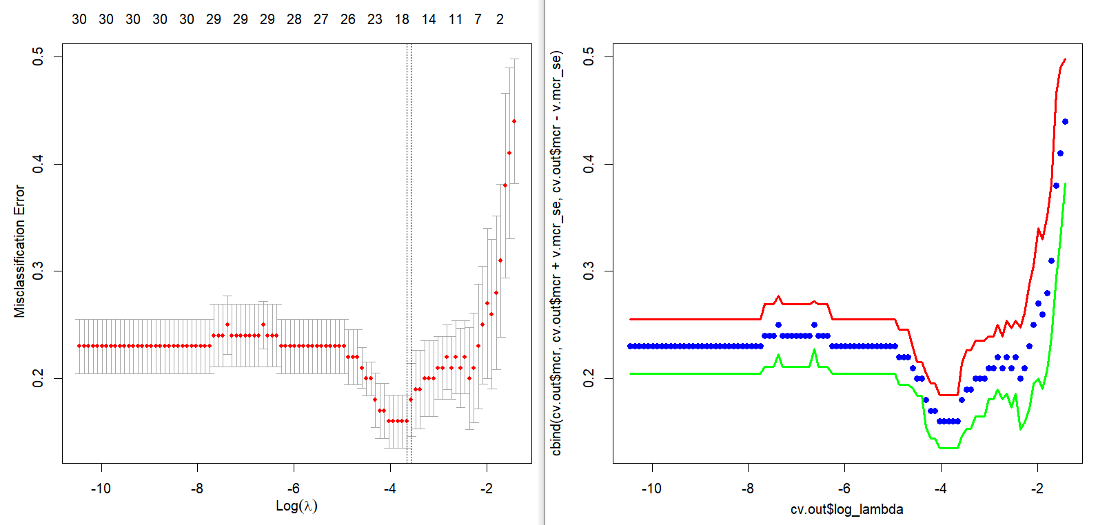
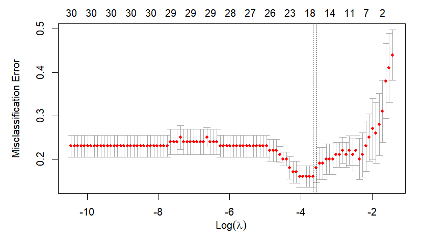
Main output of this post is the next figure. The left part is a plot for cross-validation of cv.glmnet() and the right part is the corresponding result of our calculation by hand. With this graphical output, we also calculate the above mentioned two \(\lambda\)s in the binomial context.
Cross Validation of Lasso by cv.glmnet()
K-fold cross validation (cv) generates train/test(or validation) splits across multiple folds, we can perform multiple training and testing sessions, with different splits. Now that we are familiar with k-fold cross validation, we do not repeat it redundantly in this post. Using cv.glmnet(), we can write the following R code to perform a cross validation in the lasso estimation, which is focused on a variable selection.
1 2 3 4 5 6 7 8 9 10 11 12 13 14 15 16 17 18 19 20 21 22 23 24 25 26 27 28 29 30 31 32 33 34 35 36 37 38 39 | #========================================================# # Quantitative Financial Econometrics & Derivatives # ML/DL using R, Python, Tensorflow by Sang-Heon Lee # # https://shleeai.blogspot.com #--------------------------------------------------------# # Cross Validation of Lasso : Binomial Response #========================================================# library(glmnet) library(caret) # confusion matrix graphics.off() # clear all graphs rm(list = ls()) # remove all files from your workspace set.seed(1234) #============================================ # data : x and y #============================================ data(BinomialExample) # built-in data nfolds = 5 # number of folds #============================================ # cross validation by using cv.glmnet #============================================ cvfit <- cv.glmnet( x, y, family = "binomial", type.measure = "class" , nfolds = nfolds, keep = TRUE # returns foldid ) # two lambda from cv.glmnet cvfit$lambda.min; cvfit$lambda.1se x11(); plot(cvfit) | cs |
In the above R code, we use a built-in binomial class example data (BinomialExample) for simplicity. In particular, when we set argument foldid, we can fix the grouping of folds manually. Without this argument, cv.glmnet() determines it automatically. Argument keep = TRUE makes information of grouping (foldid) available.
For a replication purpose, we reuse two vectors from a baseline lasso model
1) the range of lambda for assigning candidate \(\lambda\)s
2) the vector of fundid for identifying n-th fold
Of course, these two vectors can be user-defined.
Running the above R code results in the following two \(\lambda\)s and figure.
Calculation of lambda.min and lambda.1se
lambda.min and lambda.1se are known as recommendations of selection criteria.
Before the specific implementation, let's figure out how to calculate lambda.min and lambda.1se. It is worth noting that cross-validated errors are generated with respect to each \(\lambda\).
lambda.min : \(\lambda\) of minimum mean cross-validated error
lambda.1se : largest value of \(\lambda\) such that error is within 1 standard error of the cross-validated errors for lambda.min.
Specifically, lambda.1se is the \(\lambda\) for maximum avg(mcr) from a set of
\[\begin{align} \text{avg}(mcr) &\lt \min(\text{avg}(mcr)) + \text{se}(mcr) \\ \text{se}(mcr) &= \text{stdev}(mcr)/\sqrt{N_{fold}} \end{align}\]
where mcr denotes misclassification error rates by each \(\lambda\) and \(N_{fold}\) is the number of folds. avg(mcr) and se(mcr) are an average and standard error of mcr by each \(\lambda\).
Cross Validation of Lasso without cv.glmnet()
The following R code implements a cross validation procedure for lasso, which has the same functionality of cv.glmnet().
1 2 3 4 5 6 7 8 9 10 11 12 13 14 15 16 17 18 19 20 21 22 23 24 25 26 27 28 29 30 31 32 33 34 35 36 37 38 39 40 41 42 43 44 45 46 47 48 49 50 51 52 53 54 55 56 57 58 59 60 61 62 63 64 65 66 67 68 69 70 71 72 73 74 75 76 77 | #============================================ # cross validation by hand #============================================ # get a vector of fold id used in cv.glmnet # to replicate the same result. foldid <- cvfit$foldid # from glmnet # candidate lambda range fit <- glmnet(x, y, family = "binomial") v.lambda <- fit$lambda nla <- length(v.lambda) m.mce <- m.tot <- m.mcr <- matrix(0,nrow = nfolds, ncol=nla) #------------------------------- # iteration over all folds #------------------------------- for (i in 1:nfolds) { # training fold : tr # validation fold : va ifd <- which(foldid==i) # i-th fold tr.x <- x[-ifd,]; tr.y <- y[-ifd] va.x <- x[ifd,]; va.y <- y[ifd] # estimation using training fold fit <- glmnet(tr.x, tr.y, family = "binomial", lambda = v.lambda) # prediction on validation fold prd <- predict(fit, newx = va.x, type = "class") # misclassification error for each lambda for(c in 1:nla) { # confusion matrix cfm <- confusionMatrix( as.factor(prd[,c]), as.factor(va.y)) # misclassification count m.mce[i,c] <- cfm$table[1,2]+cfm$table[2,1] # total count m.tot[i,c] <- sum(cfm$table) # misclassification rate m.mcr[i,c] <- m.mce[i,c]/m.tot[i,c] } } # average misclassification rate (mcr) v.mcr <- colMeans(m.mcr) # save manual cross validation output cv.out <- data.frame(lambda = v.lambda, log_lambda = log(v.lambda), mcr = v.mcr) #------------------------------- # lambda.min #------------------------------- no_lambda_min <- which.min(cv.out$mcr) cv.out$lambda[no_lambda_min] #------------------------------- # lambda.1se #------------------------------- # standard error of mcr v.mcr_se <- apply((m.mce)/m.tot,2,sd)/sqrt(nfolds) # se of mcr(lambda.min) mcr_se_la_min <- v.mcr_se[no_lambda_min] # lambda.1se max(cv.out$lambda[ cv.out$mcr < min(cv.out$mcr) + mcr_se_la_min]) #------------------------------- # graph for cross validation #------------------------------- x11(); matplot(x = cv.out$log_lambda, y=cbind(cv.out$mcr, cv.out$mcr+v.mcr_se, cv.out$mcr-v.mcr_se), lty = "solid", col = c("blue","red","green"), type=c("p","l","l"), pch = 16, lwd = 3) | cs |
We can find that the following results are the same as that of cv.glmnet().
1 2 3 4 5 6 7 8 9 10 | > #------------------------------- > # lambda.min w/o cv.glmnet() > #------------------------------- [1] 0.02578548 > > #------------------------------- > # lambda.1se w/o cv.glmnet() > #------------------------------- [1] 0.02829953 | cs |
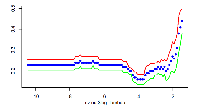
Cross validation graph is also same as that of cv.glmnet(). In the following figure, points without solid line and two solid lines denote average misclassification rates and upper/lower 1 standard error bounds respectively.
Concluding Remarks
From this post, we can 1) implement a cross validation of lasso model, 2) calculate lambda.min and lambda.1se, and 3) generate a cross validation figure. This can be extended to group lasso, exclusive lasso, and so on. Furthermore it can be easily modified to account for the case of a continuous response and time-series data. These additional extended contents will be covered in the next posts. \(\blacksquare\)


No comments:
Post a Comment