
Step-by-step refinement of R graph
This post focuses on enhancing R-generated graphs, specifically using a graph for the Nelson-Siegel-Svensson (NSS) factor loadings as an example. I employ a step-by-step approach to facilitate easy comparison of the differences in R codes, which result in slightly different graphs.
It is worth noting that this content is neither original nor highly fashioned, as I have collected these techniques from Google.
1) Default graph
We can draw the NSS factor loadings using the matplot() function without specifying any specific options, relying on the default settings.
# remove all files from your workspace graphics.off(); rm(list = ls()) nss_factor_loading <- function(la, m) { la1 <- la[1]; la2 <- la[2] C <- cbind( rep(1,length(m)), (1-exp(-la1*m))/(la1*m), (1-exp(-la1*m))/(la1*m)-exp(-la1*m), (1-exp(-la2*m))/(la2*m)-exp(-la2*m)) return(C) } #------------------------------------------------------------- # factor loading comparisons #------------------------------------------------------------- maty_ip <- c(0.000000001, 1:240/12) nf <- 4; factor_legend <- c("L","S","C1","C2") la <- c(0.07, 0.03)*12 loadings <- nss_factor_loading(la, maty_ip) #------------------------------------------------- # common graph settings #------------------------------------------------- vcol <- c(1,5,2,4); vlwd <- c(2,5,3,4); vlty <- c(1,1,2,1) str_xlab <- "Maturity in year" str_ylab <- "Factor loadings" str_main <- "NSS factor loadings" # X axis labels v_x_axis <- seq(5,max(maty_ip),5) #------------------------------------------------- # 1) Raw graph #------------------------------------------------- x11(width=6.5, height=4.5); matplot(loadings, type="l", lty=vlty, lwd=vlwd, col=vcol, xaxt = 'n', xlab = str_xlab, ylab = str_ylab, main = str_main) # x-axis labels axis(1, at = c(0,v_x_axis*12), labels = c(0, v_x_axis)) # legend legend("right",pch=16, lty=vlty, col=vcol, lwd=vlwd, cex = 0.8, bty = "n", legend=factor_legend) | cs |
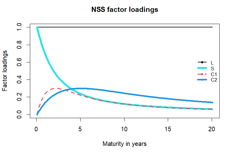
It's not bad, but some refinement would enhance it.
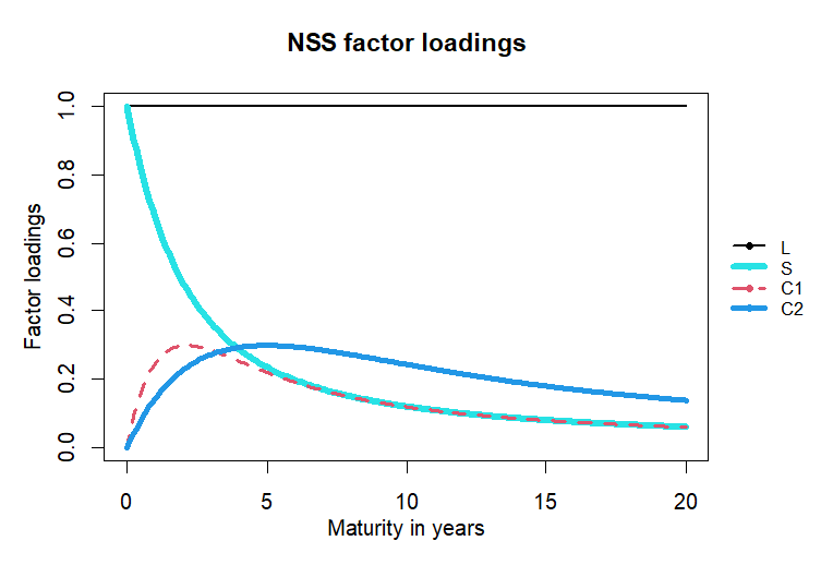
2) Some refinements and positioning the legend outside
I positioned the legend outside the plot area and moved it closer to the y-axis. Additionally, I reduced the right outer margin and adjusted the margins to bring the axis titles closer.
#------------------------------------------------- # 2) Raw graph # + position the legend outside the plot area # + move the legend more closely to the y-axis # + reduce the right outer margin # + adjust the margins to bring the axis titles closer #------------------------------------------------- right_move = -0.17 x11(width=6.5, height=4.5); par(mar = c(4, 4, 4, 5)) # bottom, left, top, right matplot(loadings, type="l", lty=vlty, lwd=vlwd, col=vcol, xaxt = 'n', xlab = "", ylab = "", main = str_main) # x, y axis labels # Adjust the margins to bring the axis titles closer # by using line = ... mtext(side = 1, line = 2, str_xlab) mtext(side = 2, line = 2.3, str_ylab) axis(1, at = c(1, v_x_axis*12+1), labels = c(0, v_x_axis)) # The inset argument controls the distance from the margins # of the plot. Adjust this value to move the legend. # xpd = TRUE --> outside legend legend("right", pch=16, lty=vlty, col=vcol, lwd=vlwd, cex = 0.8, bty = "n", legend=factor_legend, inset = right_move, xpd = TRUE) | cs |
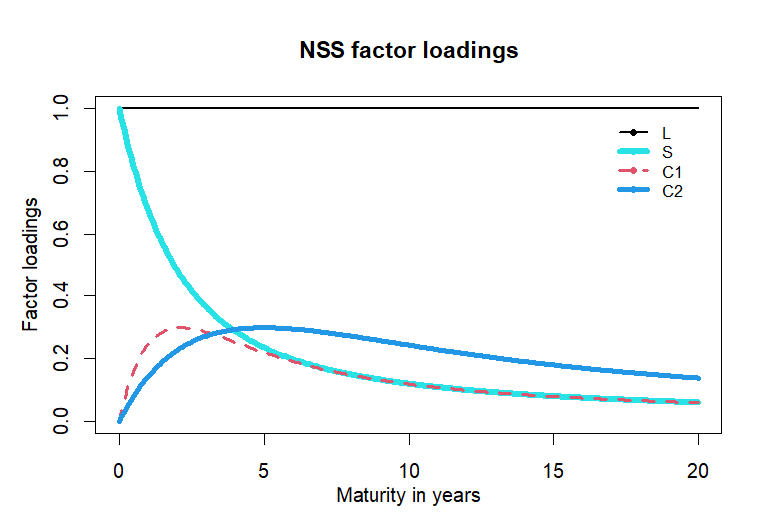
3) Positioning legend inside
We can position a legend inside without using the xpd = TRUE option.
#------------------------------------------------- # 3) Raw graph # + move the legend more closely to the y-axis # + reduce the right outer margin # + adjust the margins to bring the axis titles closer #------------------------------------------------- x11(width=6.5, height=4.5); par(mar = c(4, 4, 4, 2)) # bottom, left, top, right matplot(loadings, type="l", lty=vlty, lwd=vlwd, col=vcol, xaxt = 'n', xlab = "", ylab = "", main = str_main) # x, y axis labels mtext(side = 1, line = 2, str_xlab) mtext(side = 2, line = 2.3, str_ylab) axis(1, at = c(1, v_x_axis*12+1), labels = c(0, v_x_axis)) # do not use xpd = TRUE for inside legend legend("topright", pch=16, lty=vlty, col=vcol, lwd=vlwd, cex = 0.8, bty = "n", inset = 0.05, legend=factor_legend) | cs |
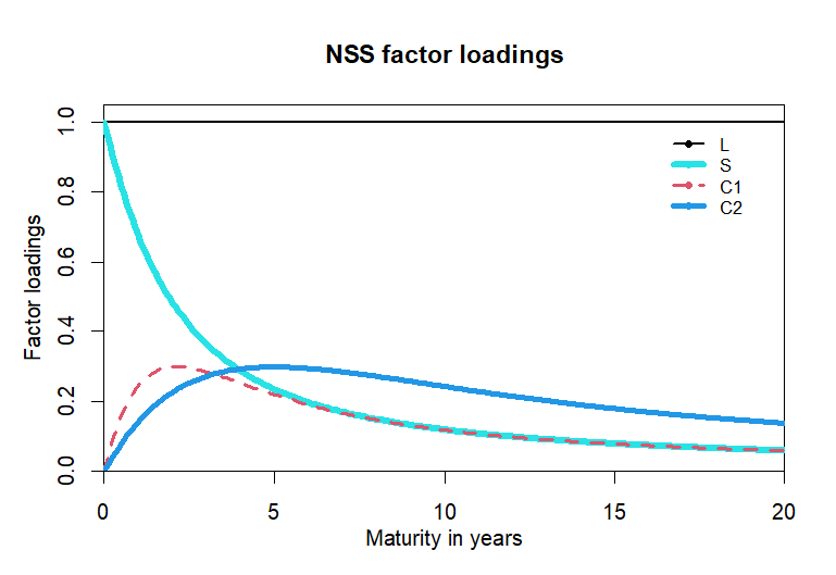
4) Fitting within the original data range
By configuring xaxs and yaxs, we can remove margins that extend beyond the minimum and maximum of each axis.
#------------------------------------------------- # 4) Raw graph # + move the legend more closely to the y-axis # + reduce the right outer margin # + adjust the margins to bring the axis titles closer # + fits within the original data range #------------------------------------------------- x11(width=6.5, height=4.5); par(mar = c(4, 4, 4, 2)) # bottom, left, top, right # You can set the xaxs and yaxs arguments to "i" # as opposed to the default of "r". From the par help page: # # Style "r" (regular ) first extends the data range by 4 percent at each end # and then finds an axis with pretty labels # that fits within the extended range. # Style "i" (internal) just finds an axis with pretty labels that # fits within the original data range. matplot(loadings, type="l", lty=vlty, lwd=vlwd, col=vcol, xaxs = "i", # fits within the original data range for x yaxs = "i", # fits within the original data range for y xaxt = 'n', xlab = "", ylab = "", main = str_main, ylim = c(0,1.05)) # x, y axis labels mtext(side = 1, line = 2, str_xlab) mtext(side = 2, line = 2.3, str_ylab) axis(1, at = c(1, v_x_axis*12+1), labels = c(0, v_x_axis)) legend("topright", pch=16, lty=vlty, col=vcol, lwd=vlwd, cex = 0.8, bty = "n", inset = 0.05, legend=factor_legend) | cs |
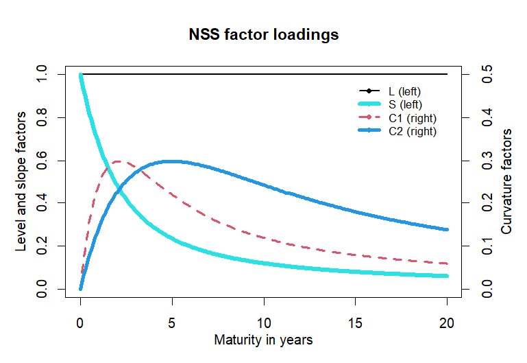
5) Two Y axes
We can utilize two y-axes by adding a second y-axis. The essential additions include par(new = TRUE) and axis(4) for this purpose.
#------------------------------------------------- # 5) Two y-axis #------------------------------------------------- x11(width=6.5, height=4.5); par(mar = c(4, 4, 4, 4)) # bottom, left, top, right # Plot the first two time series on the left y-axis matplot(loadings[,1:2], type = "l", lty = vlty[1:2], lwd = vlwd[1:2], col = vcol[1:2], xaxt = 'n', xlab = "", ylab = "", main = str_main, ylim = c(0,1)) # x, y1 axis labels mtext(side = 1, line = 2, str_xlab) mtext(side = 2, line = 2.3, "Level and slope factors") # draw graph for a second y-axis on the right side par(new = TRUE) matplot(loadings[,3:4], type = "l", lty = vlty[3:4], lwd = vlwd[3:4], col = vcol[3:4], xaxt = 'n', yaxt = 'n', xlab = "", ylab = "", main = "", ylim = c(0,0.5)) # add a second y-axis on the right side axis(4) mtext(side = 4, line = 2.2, "Curvature factors") axis(1, at = c(1, v_x_axis*12+1), labels = c(0, v_x_axis)) legend("topright", pch=16, lty=vlty, col=vcol, lwd=vlwd, cex = 0.8, bty = "n", inset = 0.05, legend=c(paste0(factor_legend[1:2]," (left)"), paste0(factor_legend[3:4]," (right)"))) | cs |
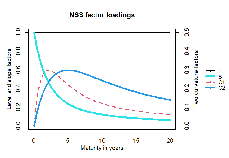
6) Two Y axes and legend outside
We can also shift a legend outside using the xpd = TRUE option.
#------------------------------------------------- # 6) Two y-axis, outside legend #------------------------------------------------- right_move = -0.35 x11(width=6.5, height=4.5); par(mar = c(4, 4, 4, 7.5)) # bltr #par(mgp = c(2, 0.7, 0)) # adjust the 1st element # Plot the first two time series on the left y-axis matplot(loadings[,1:2], type = "l", lty = vlty[1:2], lwd = vlwd[1:2], col = vcol[1:2], xaxt = 'n', xlab = "", ylab = "", main = str_main, ylim = c(0,1)) mtext(side = 1, line = 2, str_xlab) mtext(side = 2, line = 2.3, "Level and slope factors") # draw graph for a second y-axis on the right side par(new = TRUE) matplot(loadings[,3:4], type = "l", lty = vlty[3:4], lwd = vlwd[3:4], col = vcol[3:4], xaxt = 'n', yaxt = 'n', xlab = "", ylab = "", main = "", ylim = c(0,0.5)) axis(4) mtext(side = 4, line = 2.3, "Two curvature factors") axis(1, at = c(1, v_x_axis*12+1), labels = c(0, v_x_axis)) # use xpd = TRUE for outside legend legend("right", pch=16, lty=vlty, col=vcol, lwd=vlwd, cex = 0.8, bty = "n", legend=factor_legend, inset = right_move, xpd = TRUE) | cs |
There are numerous options available for creating diverse figures, but it's beyond my ability. I am only familiar with a few of them, which are presented in this post.
No comments:
Post a Comment